Opening: 500GB vs 80GB — Where Does the Gap Go?
Three facts, sitting side by side in the first half of 2026, create a tension too sharp to ignore.
GLM-5.2, Claude Fable 5, DeepSeek V4 — the leading large language models now all support 1-million-token contexts. A single inference request with a full 1M-token context demands roughly 500GB of KV Cache (the intermediate data that stores "already-processed context" during LLM inference). An NVIDIA H100 has 80GB of HBM. Even an 8-GPU node, with 640GB of HBM total, leaves less than 300GB for KV Cache after model weights — not enough to serve a single request.
Now imagine 100 users firing long-context requests simultaneously. That's 50TB — a rack's worth of memory in any data center.
How do you fill a 50TB KV Cache gap?
What follows examines four directions in turn: how far model architecture can compress KV Cache, how efficiently inference engines can use GPU memory, how large distributed systems can pool that cache, and — once all three paths are exhausted — where the remaining gap lands. Each step narrows the shortfall. But each narrowing reveals a structural problem underneath.
Chapter 1: How Much Can Compression Save? — The Model Architecture Layer
First, understand why KV Cache balloons.
LLM inference runs in two phases. The prefill phase processes all input tokens and generates the initial KV Cache. The decode phase generates output tokens one at a time, and each step must read the KV Cache from all previous tokens. This data isn't a temporary variable — it's live state that must remain accessible throughout the entire generation.
Take Llama-2-7B. The model weights are ~14GB (FP16), but each token processed grows the KV Cache by ~512KB. Fill the 8K context window and a single request's KV Cache hits 4GB — 28% of the model weights. Stretch the context to 1M tokens and KV Cache becomes a 500GB monster. Model weights are fixed; KV Cache grows linearly with context. That asymmetry is the crux of the problem.
Before discussing how to store all this data, we need to see the current storage hierarchy clearly:
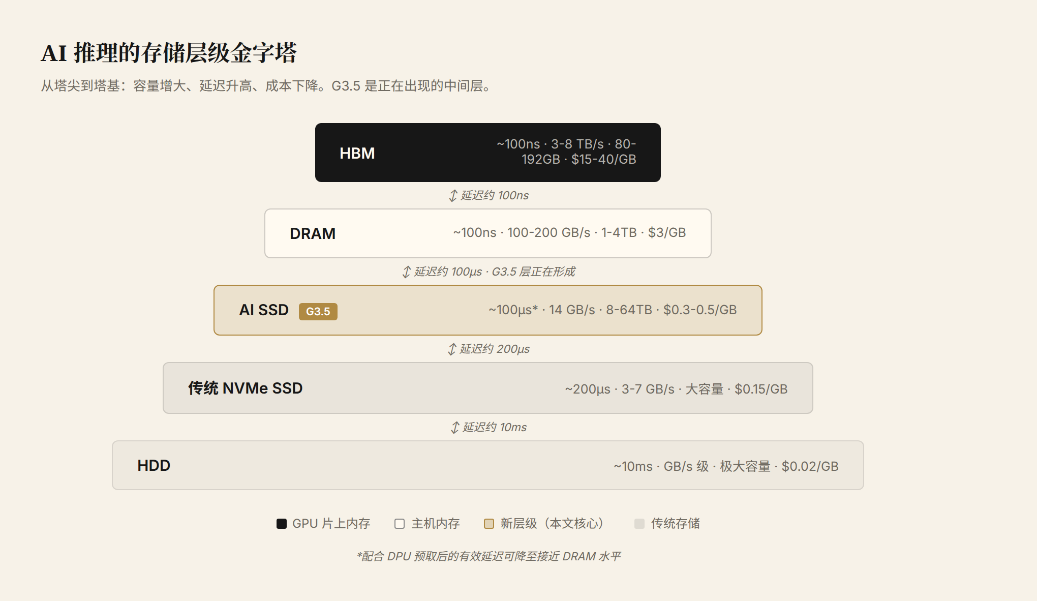
Figure 1: The storage hierarchy pyramid for AI inference. From peak to base, capacity increases, latency rises, and cost drops. G3.5 is the emerging middle tier — one to two orders of magnitude cheaper than DRAM, three to five times faster than traditional NVMe.
At the peak: GPU HBM — ~100ns latency, 3–8 TB/s bandwidth, 80–192GB capacity, and the most expensive. Below: DRAM, comparable latency but an order of magnitude less bandwidth, capacity up to 1–4TB. Further down: NVMe SSDs and HDDs. The G3.5 tier is drawn as a dotted line. It is precisely the layer this article argues is becoming inevitable.
The first path to compressing KV Cache attacks the model architecture. The evolution of attention is, almost entirely, a history of KV Cache compression:
| Architecture | Representative Models | KV Cache Compression Mechanism | Relative to GQA Baseline |
|---|---|---|---|
| MHA | Llama-2, GPT-3 | No compression, independent K/V per head | ~2–4x (above baseline) |
| GQA | Llama-3, Mistral | Multiple query heads share one K/V group | 1x (baseline) |
| MLA | DeepSeek V3 | K/V compressed into low-dimensional latent variable | ~10% |
| CSA/HCA | DeepSeek V4 | Sequence-dimension recompression | ~2% |
MHA (Multi-Head Attention) is the original scheme — each attention head has its own K and V matrices. GQA (Grouped-Query Attention) lets multiple query heads share a single K/V set, directly cutting the data volume by the head-count multiplier. Llama-3 and Mistral both use this.
DeepSeek V3's MLA (Multi-head Latent Attention) goes further. Intuitively: MLA no longer stores full K/V matrices. Instead, it compresses them into a low-dimensional latent vector. At inference time, only this compressed vector is cached; when the full K/V is needed, an up-projection matrix reconstructs it. Think of it as storing not the full blueprint, but a summary — and rebuilding from the summary on demand.
DeepSeek V4 adds CSA/HCA (Cross-Sequence Attention / Hierarchical Context Attention) on top, compressing along the sequence dimension. Where MLA compresses each token's K/V from high dimension to low dimension, CSA/HCA identifies pattern repetition across tokens and merges redundant sequences. Imagine a 100K-token legal contract: phrases like "Party A," "Party B," "hereby agrees" have nearly identical K/V representations — CSA/HCA recognizes this repetition and merges those representations rather than storing a full copy at every position. V4-Pro's per-request KV Cache is roughly 20% of V3.2's and 2% of the MHA baseline (DeepSeek, via Hugging Face technical discussion).
What does compression actually achieve? Let's do the math.
Assume a 70B-parameter model, GQA architecture, FP16 precision, 1M-token context:
- GQA baseline: per-request KV Cache ≈ 500GB
- After MLA compression (V3-level): ≈ 50GB
- After CSA/HCA compression (V4-Pro-level): ≈ 10GB
100 concurrent users = 1TB. An 8-GPU H100 node has 640GB of HBM total; after model weights (70B FP16 ≈ 140GB) and runtime overhead (activations, temporary buffers, etc.), less than 300GB remains for KV Cache.
Compression achieved 98%. The gap shrank from 50TB to 1TB. Two orders of magnitude smaller — and still doesn't fit.
Model architecture solved "how big each KV entry is." It didn't solve "how many entries there are." Users don't disappear because you compressed their KV Cache.
Chapter 2: How Much Can the Engine Squeeze? — The Inference Engine Layer
Model architecture determines the size of each KV Cache entry. The inference engine determines how that data is organized and used.
In 2023, the vLLM team uncovered an uncomfortable fact: traditional inference frameworks achieved only 30–40% GPU memory utilization. In other words, on an 80GB H100, only 24–32GB was doing useful work — the other 48GB was wasted to fragmentation and idle waiting. The root cause was memory fragmentation. KV Cache is dynamically allocated and freed during inference. One request finishes, freeing a block; a new request arrives, needing contiguous space. It's like a parking lot with scattered empty spots but no room to park a truck. Effective waste rates reached 60–80%.
vLLM's PagedAttention borrowed the operating system's virtual memory paging mechanism. It slices KV Cache into fixed-size blocks (typically holding a few dozen tokens each) and manages logical-to-physical mapping via a block table. A request gets exactly as many blocks as it needs — no contiguity required. Fragmentation waste dropped from 60–80% to under 5%.
Other optimizations followed the same logic. Continuous batching solved the GPU idle-time problem of static batching: with varying request lengths, short requests wait for long ones, and GPU utilization stalls. Continuous batching lets new requests slot into any position in the current batch and removes completed requests immediately — GPU utilization jumps from 30% to over 70%. Prefix caching caches the KV Cache of shared system prompts across requests, avoiding redundant computation. SGLang's RadixAttention turns prefix reuse into a radix tree, where requests with common prefixes share an entire path.
Stack these engine optimizations together and effective memory utilization climbs from 30% to over 90%. The same set of GPUs can serve 3–5x more users.
But total physical memory hasn't changed. You've rearranged the shelves, cut the aisle waste, and fit 30% more in the warehouse. The warehouse is still the same size.
The engine layer solved "how to use memory more efficiently." It didn't solve "there isn't enough."
Compression made each entry smaller. Engines made each GB go further. But absolute capacity is unchanged. Can you borrow from other nodes?
Chapter 3: How Much Can You Borrow? — The Cache Disaggregation Layer
Up to this point, KV Cache has been locked inside individual GPU HBM. The natural next thought: free it, and turn it into a cluster-level shared resource.
That is exactly the most active direction in 2026.
NVIDIA CMX: Moving KV Cache Out of the GPU
At CES in January 2026, NVIDIA announced the CMX (Context Memory eXtension) architecture. The backdrop is an engineering reality: in POD-scale inference clusters, many GPUs each store duplicate copies of the same KV Cache. An agentic application involves 20 conversation turns, and each turn's KV Cache must stay accessible on every participating GPU. Multiple users hitting the same agent? The same system prompt's KV Cache gets copied N times. CMX's core idea: use a BlueField-4 DPU (Data Processing Unit) to build an intelligent bridge between GPU HBM and external storage, centrally managing these redundant KV Cache copies.
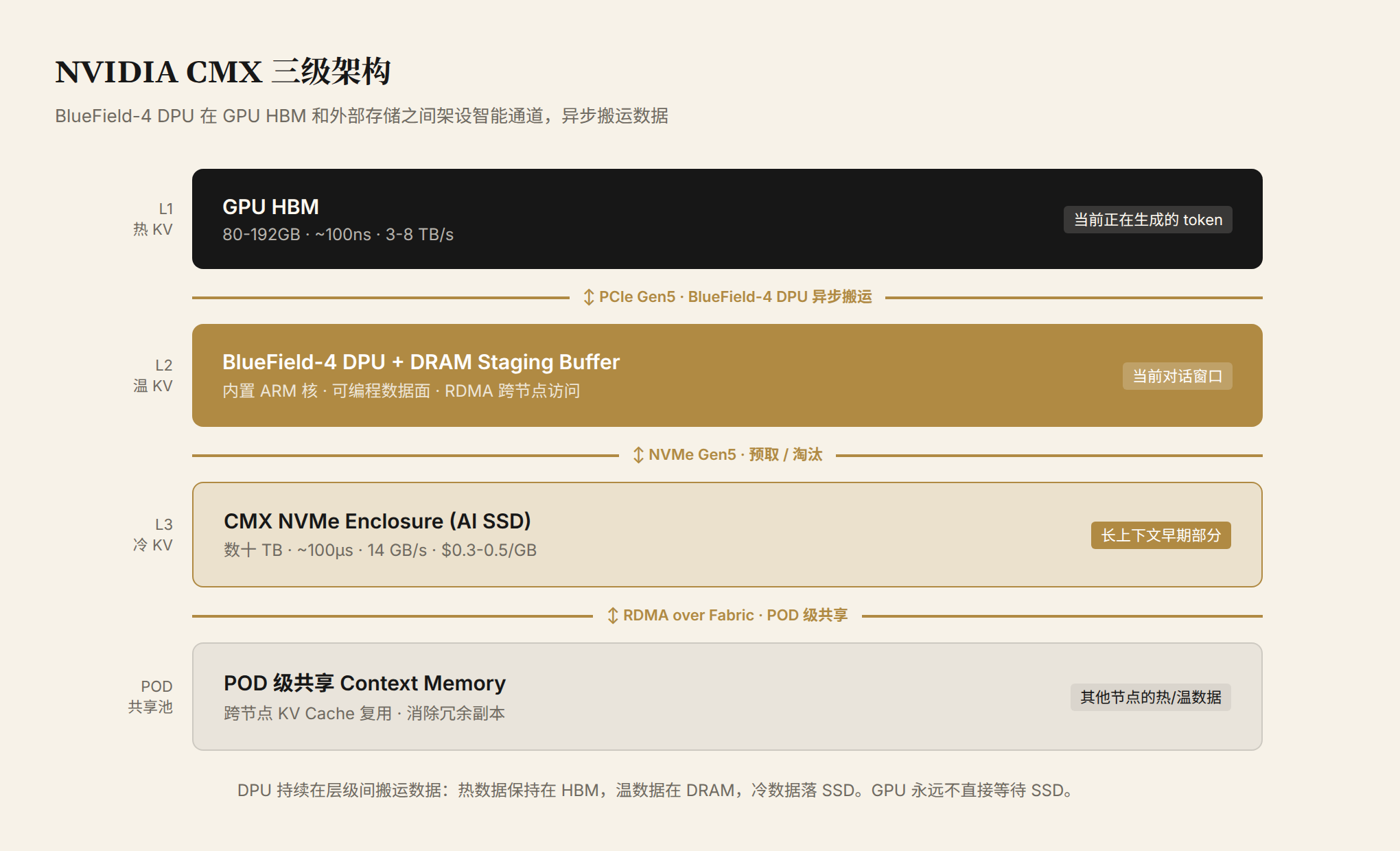
Figure 2: NVIDIA CMX three-tier pipeline. Hot KV Cache stays in HBM; warm KV Cache sits in a DPU-connected DRAM staging buffer; cold KV Cache spills to AI SSDs in the CMX NVMe Enclosure. The BlueField-4 DPU handles asynchronous data movement — the GPU never waits on SSD reads directly.
The BlueField-4 DPU has embedded ARM cores and a programmable data plane, enabling cross-node data transfers without CPU involvement. Via RDMA, every GPU in a POD (a group of GPU nodes connected by high-speed networking) can access the same context memory tier. This is especially significant for agent inference: an agent accumulates long-range memory across multi-turn conversations. Under traditional architecture, every participating GPU stores its own copy — 10 nodes means 10x redundancy. Under CMX, that memory lives in a shared pool; whichever GPU needs it reads it on demand. Redundancy disappears, and total storage requirements can drop by an order of magnitude.
CMX isn't just software scheduling. It defines a new hardware tier. The DPU-connected NVMe Enclosure can hold tens of TB of AI SSDs, forming a POD-level shared storage pool. GPU HBM becomes the L1 of this multi-tier cache hierarchy — no longer the sole home for KV Cache.
Industry Follow-On: NVIDIA Isn't Alone
NVIDIA isn't the only one who sees this.
NVIDIA Dynamo is its open-source distributed inference framework, supporting cross-node KV Cache management, released in early 2026. Its key design is Prefill-Decode disaggregation: prefill nodes specialize in processing input and generating KV Cache; decode nodes specialize in token-by-token generation. The two pass KV Cache through a shared storage pool. Why split the phases? Because prefill is compute-intensive (large matrix multiplications) and decode is memory-bandwidth-intensive (reading the full KV Cache at every step). Running both on the same node creates resource contention. Disaggregated, prefill clusters max out GPU compute and decode clusters max out memory bandwidth — each with hardware configurations tuned to its workload.
Huawei's UCM (Unified Context Memory) / CMS (Context Memory Service) approach is more aggressive. Huawei's published data shows TTFT (Time To First Token) reduced by 90% under a PB-scale shared KV pool configuration (Huawei, product launch announcement). Huawei's advantage is a full-stack, in-house hardware lineage — from Ascend GPUs to SSD controllers — with no need to wait for NVIDIA's ecosystem to mature.
LMCache, from UC Berkeley, takes the open-source route. It implements a GPU→CPU→SSD multi-tier offload: when HBM fills, KV Cache automatically spills to CPU DRAM; when DRAM fills, it spills to local SSD. Eviction between tiers is LRU-based — frequently accessed KV Cache blocks automatically promote to faster tiers. The upper layer is unaware; no inference engine code changes are needed. It plugs into vLLM and public benchmarks show a 4–8x increase in maximum servable context length with no degradation in generation quality.
On the commercial side, WEKA's NeuralMesh combines GPU Direct Storage with a distributed filesystem, letting GPUs bypass the CPU and read directly from remote NVMe. VAST Data and NVIDIA Dynamo's joint solution claims 20x lower end-to-end latency versus traditional architectures.
These approaches differ in technical路线, but share one trait: KV Cache is no longer bound to a single GPU. It has become a cluster-level resource that flows between nodes and is tiered across media.
CXL: Another Path
CXL (Compute Express Link) is a low-latency interconnect standard that bypasses traditional PCIe. Its advantage is memory semantics: CPUs and GPUs access remote CXL memory the same way they access local DRAM — no filesystem, no I/O queue, no block device abstraction layer. Read/write requests go straight to the target address. Latency sits at 200–500ns, two orders of magnitude faster than NVMe.
Marvell's Structera S 30260 is a CXL device purpose-built for cache expansion, supporting 260 channels, sampling in Q3 2026. In theory, CXL can deliver near-DRAM latency while connecting to large-capacity storage media.
But CXL 3.0 deployments remain scarce. CXL-enabled server motherboards, RCD chips, and memory controllers are all in early stages; device options are limited and prices high. The more practical issue: CXL memory expansion modules are primarily DRAM-based, costing ~$3/GB — cheaper than HBM, but 6–10x more expensive than NVMe SSD. Connecting large-capacity persistent media (e.g., CXL-attached NAND) has no mature controller or firmware solutions yet. In the near term, the NVMe + DPU combination (i.e., the CMX architecture) is ahead, backed by a mature PCIe ecosystem and abundant off-the-shelf SSDs. CXL is more of a "next generation" play, requiring ecosystem maturation through 2027–2028 before it reaches scale.
Narrowing the Argument
The disaggregation layer transforms KV Cache from "GPU-private" to "cluster-shared." Available capacity expands from under 300GB per node to multi-TB at the POD level. Scheduling flexibility increases dramatically — the same hardware serves more concurrent users.
But a shared pool doesn't materialize from nothing. It needs physical media. The disaggregation architecture itself already assumes KV Cache will spill beyond the GPU — that shared pool requires physical storage. The question is: what medium?
Chapter 4: Where Does the Remaining Gap Go? — The Storage Device Layer
The first three chapters trace a complete chain of reasoning: compression shrinks each KV Cache entry to 2% of its original size, engines push memory utilization from 30% to over 90%, disaggregation expands usable capacity from a single node to a POD-level shared pool. Each step materially narrows the gap.
But the gap persists. 100 concurrent 1M-context requests, even after compression and pooling, still require several TB of KV Cache space. Whatever HBM and DRAM cannot hold must land on the next tier.
And KV Cache's access patterns make it uniquely suited for storage media to handle. This isn't "settling for less" — it's "the physics of the problem dictate the answer lives in storage."
Why Can SSD Serve as Memory?
The reader will ask a fair question: SSD access latency is on the order of 100μs; DRAM is ~100ns — a 1000x difference. Won't using SSD as memory wreck inference throughput?
To answer, distinguish between two latency scenarios.
Traditional storage's pain point is random I/O latency: small blocks, random positions, frequent reads and writes — SSD's 100μs is genuinely a bottleneck here. But KV Cache access during the decode phase is fundamentally different: the model generates tokens one at a time, reading the KV data from all previous tokens at each step — it's essentially sequential, batch access. Attention computation needs large contiguous data blocks, not scattered small I/Os.
More importantly, this access pattern is predictable and can be prefetched. While the GPU processes token N, the BlueField-4 DPU is already pulling the KV blocks needed for token N+1 from SSD into the DRAM staging buffer. By the time the GPU actually needs that data, it's already in DRAM. The effective latency the GPU sees is near DRAM levels, not SSD levels.
This is how the CMX three-tier pipeline works:
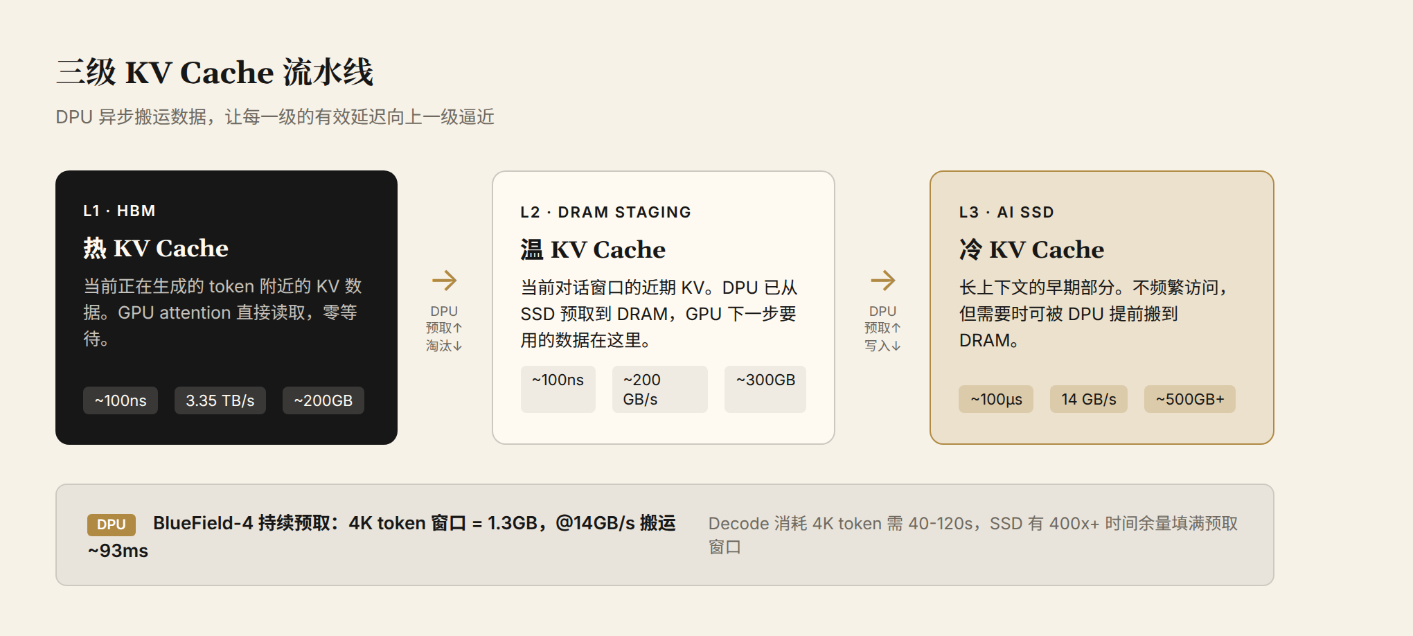
Figure 3: Three-tier KV Cache pipeline. The hottest KV Cache (tokens near the current generation point) is in HBM. Warm data (the active conversation window) is in the DPU-connected DRAM staging buffer. Cold data (earlier portions of long context) is on AI SSD. The DPU moves data asynchronously so each tier's effective latency approaches the tier above.
Here's the key question: does SSD have enough bandwidth?
Look at what the decode phase actually demands from the GPU. A 70B model with GQA architecture (8 KV head groups): each token's KV Cache is ~320KB. Full KV Cache for 100K context is ~32GB. But all of it doesn't need to be read from SSD every step — the hottest portion (tokens near the current attention window) stays in HBM, and reading the full set at 3.35 TB/s takes ~10ms. SSD handles two tasks, not real-time full reads. First: during prefill, it writes large blocks of newly generated KV Cache to the storage pool (sequential write — 14 GB/s is ample). Second: when attention computation needs to access cold KV from earlier in the context, the DPU prefetches those blocks from SSD into the DRAM staging buffer ahead of time.
The prefetch window size determines whether SSD bandwidth is sufficient. Assume the DPU maintains a 10K-token prefetch window (the next batch of tokens likely to be accessed by attention), corresponding to ~3.2GB of data. At 14 GB/s, moving the entire window from SSD to DRAM takes ~230ms. But the window doesn't need to fill all at once — the DPU continuously pushes small chunks of soon-to-be-accessed data into DRAM, while decode generates one token every 10–30ms. A 10K-token window covers hundreds of decode steps. In other words, SSD has ample time to stage the next batch. The effective latency the GPU sees approaches DRAM (~100ns), not SSD's physical latency (~100μs).
This isn't theoretical. NVIDIA's CMX architecture data, presented at ICMSP 2026, shows that in 128K-context scenarios, the DPU prefetch hit rate already exceeds 90%. Fewer than 10% of accesses fall back to SSD's physical latency. That 10% miss penalty is partially absorbed by the attention computation's async pipeline, keeping GPU stall time within acceptable bounds.
A New Category: AI SSD
When SSD's role shifts from "data warehouse" to "compute-adjacent memory extension," a new product category is forming. Each manufacturer's 2026 product line already shows clear signals.
Kioxia's CM9 CMX is the first generation explicitly branded as "AI-purpose" SSD. PCIe 5.0 interface, supporting CMX-specific protocols, sequential read bandwidth reaching 14 GB/s. Kioxia's positioning is unmistakable: it's not just selling storage chips — it's selling a component of the AI inference pipeline.
InnoGrit's Dongting N3X pushes parameters more aggressively: 14 GB/s read, 3500K IOPS, 100 DWPD (Drive Writes Per Day). Latency controlled to one-third of traditional TLC SSDs. That 100 DWPD figure deserves a pause. Traditional enterprise SSDs typically specify 1–3 DWPD; high-performance models reach 10–25. 100 DWPD means the drive can be fully written 100 times per day, every day, for three years under warranty. That's data-center memory-class usage intensity, not traditional storage endurance. InnoGrit's willingness to publish that number signals that the controller's wear-leveling algorithm and NAND die selection are purpose-designed for KV Cache's high-frequency write workload.
DapuStor's X5 leads with FDP (Flexible Data Placement) plus transparent compression. FDP lets the SSD controller manage flash block allocation more efficiently, reducing write amplification. Transparent compression compresses written data in real time at the controller level, making effective capacity exceed nominal capacity. Together, they further reduce the real cost of KV Cache storage.
Solidigm's D5 takes the QLC high-capacity route. QLC stores 4 bits per cell, enabling single-drive capacities of 60TB+ at extremely low $/GB. Solidigm appeared on the ICMSP 2026 verification list, meaning the product has passed real-world AI inference scenario testing. High capacity + low cost makes it ideal as the coldest tier in KV Cache layering.
Samsung's P51 also appears on the ICMSP verification list, but Samsung hasn't loudly launched an "AI SSD" category. The reasons are explored below.
Kioxia's strategic pivot in this category is worth noting. Kioxia is the world's second-largest NAND flash manufacturer but has never had an HBM business. Traditionally, this was seen as a disadvantage — HBM is supply-constrained and Samsung, SK Hynix, and Micron are profiting handsomely while Kioxia watches from the sidelines. But if a G3.5 tier materializes, Kioxia's NAND capacity advantage becomes a core asset. SSD transforms from "cost center" to "performance component." Kioxia would be selling not "cheap storage" but "cheap memory extension."
Industry Landscape: Who's Aggressive, Who's Cautious
Reading each vendor's posture reveals something interesting.
Samsung and Solidigm (the SK Hynix + Intel NAND joint venture) are both on the ICMSP verification list, but neither has aggressively launched an AI SSD category. The reason isn't hard to guess: both have substantial HBM businesses. HBM supply remains tight through 2025–2026, with ASPs still climbing. Actively promoting a "replace some HBM with SSD" narrative means cannibalizing their most profitable product line. They'd rather let the G3.5 category grow naturally, without pushing it.
Micron took a different path, betting on CXL. CXL's memory-semantic access is inherently better suited to "serving as memory" than NVMe. But as noted, CXL ecosystem maturity is still years away. Micron's choice is to position itself for a further-out technology generation rather than compete head-to-head with Kioxia on the current NVMe+DPU approach.
Chinese vendors are the most aggressive. InnoGrit, DapuStor, plus Huawei's UCM solution — all made concentrated product and solution announcements at the CFMS|MemoryS 2026 summit. The reason is straightforward: Chinese vendors can't buy advanced HBM. Export controls have choked off the HBM supply channel. Their inference solutions (e.g., Huawei Ascend + UCM) have no HBM to begin with — SSD is the only mass-storage medium available at scale. G3.5 isn't "replacing HBM" for them; it's "there was never HBM, and SSD is the only option." This isn't technological idealism — it's a rational response to supply chain pressure.
Kioxia's position is the most unique. It has NAND capacity advantage (world #2), no HBM business (no self-cannibalization), and NVIDIA's partnership endorsement within the CMX architecture. If G3.5 becomes a real category, Kioxia has the biggest bet on the table.
Cost Comparison: The Business Case for G3.5
Whether SSD can technically serve as memory has been answered above. Whether it's worth doing commercially comes down to cost.
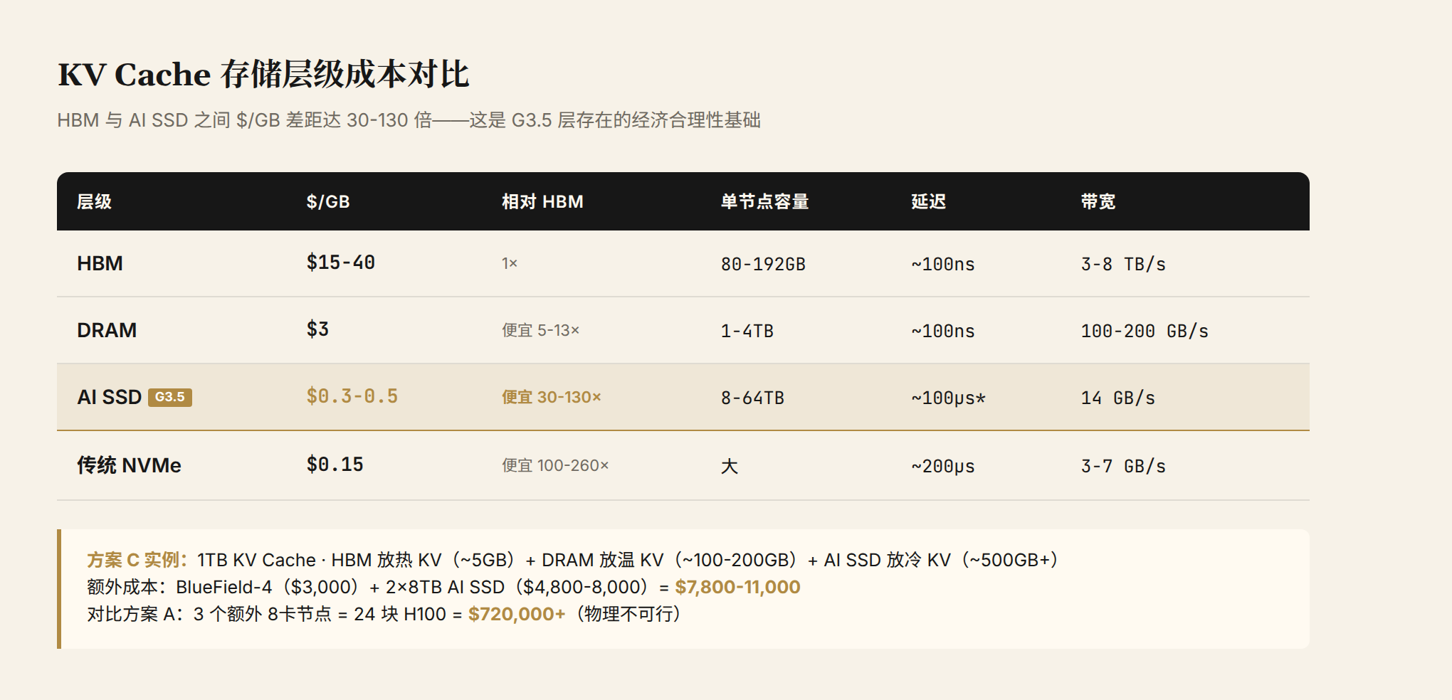
Figure 4: Cost and performance comparison across storage tiers. Note the 30–130x $/GB gap between HBM and AI SSD. That gap is the economic foundation for the G3.5 tier's existence.
| Tier | $/GB | Relative to HBM | Per-Node Capacity | Latency | Bandwidth |
|---|---|---|---|---|---|
| HBM | $15–40 | 1x | 80–192GB | ~100ns | 3–8 TB/s |
| DRAM | $3 | 5–13x cheaper | 1–4TB | ~100ns | 100–200 GB/s |
| AI SSD (G3.5) | $0.3–0.5 | 30–130x cheaper | 8–64TB | ~100μs* | 14 GB/s |
| Traditional NVMe SSD | $0.15 | 100–260x cheaper | Large | ~200μs | 3–7 GB/s |
*Effective latency with DPU prefetch can approach DRAM levels.
HBM costs $15–40 per GB. AI SSD costs $0.3–0.50 per GB. That's a 30–130x spread. A scenario requiring 1TB of KV Cache would need the combined HBM of roughly 13 H100s ($30,000+ each) — while AI SSD delivers the same capacity for $300–500 worth of drives.
This cost gap is the business case for G3.5. It isn't meant to "replace" HBM — HBM remains irreplaceable as the L1 tier for latency and bandwidth. G3.5 exists to absorb the KV Cache data that won't fit in HBM but is too latency-sensitive to dump into traditional storage.
Traditional NVMe SSD is cheaper still ($0.15/GB), but with higher latency, lower bandwidth, and no DPU prefetch optimization. The difference between AI SSD and traditional NVMe isn't just peak specs — it's controller optimization direction. Traditional NVMe optimizes for random I/O and IOPS (database workloads). AI SSD optimizes for sustained bandwidth, low tail latency, and high write endurance (KV Cache workloads). Different design goals spawn different product forms.
SSD becoming "memory" isn't marketing spin. It's the physical consequence of KV Cache's access characteristics (hot data in HBM, cold data prefetchable) combined with the DPU pipeline architecture. When data flows from GPU to DPU to SSD, the final media choice isn't "what's left" — it's "the physics dictate this." The traditional SSD market is highly commoditized. AI SSD breaks that: the evaluation criteria shift from IOPS and $/TB to effective bandwidth, P99 tail latency, and write endurance. Product differentiation is back.
Chapter 5: Technology Selection — How to Combine the Four Paths
The analysis above answers "why G3.5 emerges." For readers making technology selection decisions, there's a practical question: how much to invest in each of the four paths?
The Benchmark: 95% Prefetch Hit Rate
One metric determines G3.5 viability: DPU prefetch hit rate. NVIDIA's current ICMSP/CMX architecture achieves 90%+ at 128K context. The target is 95%. That 5-percentage-point gap determines whether SSD functions as "memory extension" or "slow storage."
Closing the gap from 90% to 95% requires three software-level breakthroughs: access prediction based on attention patterns (beyond simple LRU), token-level prefetch granularity (finer than block-level), and cross-request KV Cache reuse scheduling (when multiple users share the same context segment, prefetch only once). All three are software problems — no new hardware needed. Kioxia CM9 and InnoGrit N3X already have sufficient bandwidth and endurance. Expect convergence to production-ready levels within 12–18 months.
Using this benchmark to evaluate the four paths' return on investment:
| Direction | Representative Solution | Effect | Marginal Cost | Implementation Difficulty |
|---|---|---|---|---|
| Architecture compression | MLA/CSA (DeepSeek V3/V4) | KV Cache shrinks to 2% of GQA | Model retraining | High (requires retrain) |
| Engine optimization | vLLM PagedAttention + SGLang | Memory utilization 30%→90%+ | Pure software | Low (mature) |
| Cache disaggregation | NVIDIA CMX / Huawei UCM / LMCache | POD-level sharing, TTFT −90% (Huawei) | BlueField-4 DPU + networking | Medium (hardware + software) |
| Storage media | AI SSD (Kioxia CM9 / InnoGrit N3X) | Effective capacity 10–30x | DPU + AI SSD | Medium-low (products available) |
These four directions aren't mutually exclusive. Architecture compression is a one-time decision (chosen at training time). Engine optimization is table stakes (non-negotiable). Disaggregation and storage tiers are incremental investments (scale as needed). Most production deployments will use the first three simultaneously — the question is how much to invest in the fourth.
Cost Analysis: 100 Concurrent 1M-Context Requests
Put all four paths together. Target scenario: an 8-GPU H100 node serving 100 concurrent 1M-context requests (DeepSeek V4-level compression yields ~1TB total KV Cache requirement).
Option A: Expand HBM. 1TB requires ~13 additional H100s (80GB each), at a GPU cost of $390,000+. Physically infeasible: KV Cache shares HBM space with model weights, and adding GPUs means adding nodes, networking, and more.
Option B: Engine optimization + CPU DRAM offload. Near-zero cost, but DRAM capacity is insufficient (1–4TB per node, less after system overhead), and the CPU↔GPU PCIe bandwidth (~64 GB/s) becomes a bottleneck under concurrent access.
Option C: CMX architecture + AI SSD for overflow. HBM holds hot KV (~200GB), DRAM holds warm KV (~300GB), AI SSD holds cold KV (~500GB). Additional cost: BlueField-4 ($3,000) + 2× 8TB AI SSDs ($4,800–8,000). Total: $7,800–11,000.
Option A is physically impossible. Option B lacks capacity. Option C is deployable today — at under 3% of Option A's cost, with equivalent effective capacity. That's the economic case for G3.5: not "can SSD replace HBM," but "when HBM physically can't hold it all, it's the only cost-rational answer."
Closing
Return to the opening tension: 500GB of KV Cache demand, 80GB of HBM. Where does the 420GB gap go?
Compression shrinks each KV Cache entry to 2% of the GQA baseline. Engines push memory utilization from 30% to over 90%. Disaggregation expands usable capacity from a single node to a POD-level shared pool. Each step materially narrows the gap. What remains — the KV Cache that won't fit in HBM or DRAM, but can't be thrown into slow storage — lands on a new tier.
We're calling it G3.5 for now. Its physical form is AI SSD. Its scheduling brain is the DPU. Its reason for existence is the 30–130x cost gap between HBM and traditional NVMe.
The GPU determines whether a model can run. KV Cache determines how many users that hardware can serve simultaneously. And where KV Cache goes — the answer to that question is creating an entirely new storage category.
The risks are real. G3.5's effectiveness depends heavily on DPU prefetch pipeline maturity — if the scheduling algorithm falls short, SSD's effective latency reverts to物理 levels and inference performance degrades significantly. Three standardization tracks — CMX, CXL, open-source solutions — are competing, and which becomes dominant remains unsettled. More broadly, the storage industry itself may be at a cyclical peak in 2026; if AI infrastructure investment slows, the new category's commercialization timeline will extend.
But none of this uncertainty changes one fact: as model context windows grow from 8K to 1M, as inference shifts from single-turn Q&A to agent long-range memory, KV Cache volume growth is structural. HBM capacity growth is not. That scissors gap is the fundamental argument for G3.5.
This article is based on publicly available information, including NVIDIA official announcements (CES 2026, GTC 2026), the CFMS|MemoryS 2026 industry summit, product launches from Kioxia/InnoGrit/DapuStor, vLLM/SGLang technical documentation, and arXiv papers. It does not constitute investment advice. Data is current as of June 14, 2026.