Opening: 500GB vs 80GB
In the first half of 2026, mainstream large models pushed their context windows to 1 million tokens. GLM-5.2, Claude Fable 5, DeepSeek V4 — all natively support 1M context. How much space does KV Cache (the intermediate data storing "already-processed context" during inference) require for a single 1M-context request? Take Llama-3-70B as an example: roughly 320 GB. An NVIDIA H100 has only 80 GB of HBM. An 8-GPU node totals 640 GB of HBM; subtract model weights, and the space left for KV Cache is under 300 GB — not enough for a single request.
What about 100 users simultaneously sending long-context requests? 100 × 320 GB = 32 TB. In any data center, that is an entire rack of GPU memory.
How do you close a 32 TB KV Cache gap?
You cannot brute-force it with more GPUs. HBM costs $15–40 per GB. 32 TB means hundreds of millions of dollars in memory alone. The real answer is a five-layer optimization chain: model architecture compresses the size of each KV Cache; precision encoding halves it again; inference engines push GPU memory utilization from 30% to 90%; cluster architecture lets KV Cache flow across nodes; and storage devices use SSDs to absorb spilled cold data. Each layer shrinks the gap — and each shrinkage exposes the structural problem of the next layer.
DeepSeek V4 demonstrates the ultimate potential of this chain. Through its four-stage hybrid compressed attention, V4-Pro's KV Cache for a single 1M-context request is only 9.62 GB — 3% of an equivalent GQA scheme. Stack FP8 precision, Prefix Caching, and Prefill-Decode disaggregation on top, and the effective KV footprint per request drops below 1 GB.
This article dissects the optimization chain layer by layer, concluding with an economic model and decision framework for 1,000-GPU clusters.
Chapter 1: The Nature of KV Cache — Why It Matters More Than FLOPS
Two-Phase Inference
Large model inference runs in two phases.
The Prefill phase processes the user's entire input token sequence. The model generates K (Key) and V (Value) matrices for every attention layer and writes them to a cache. A 100K-token input generates 100K KV entries in a single prefill pass. This phase is compute-bound: GPU FLOPS are fully saturated, and each token's KV Cache is written exactly once.
The Decode phase generates output tokens one at a time. For each new token, the model reads the entire KV Cache of all previous tokens to perform attention — it "looks back" at the full history. This phase is memory-bound: the computation is just one attention layer, but the full KV Cache must be repeatedly read. The bottleneck is memory bandwidth and capacity.
KV Cache exists to avoid redundant computation. Without it, generating the Nth token requires recomputing attention for all preceding N−1 tokens — O(N²) cost. With KV Cache, each step only computes the new token's K/V, stores it, and performs one attention pass — O(N). In practice, on a HuggingFace T4 GPU, using KV Cache is 5.2× faster than not (11.7s vs 61s).
How Big Is KV Cache?
The precise formula:
Per-token KV Cache = 2 × n_layers × n_kv_heads × d_head × precision_bytes
2: Key and Value, one copy eachn_layers: number of model layersn_kv_heads: number of KV heads (far fewer than query heads after GQA)d_head: dimension per headprecision_bytes: bytes per value (FP16=2, FP8=1, INT4=0.5)
Plugging three mainstream 2026 models into the formula reveals just how wide the gap can be.
Llama-3-70B (GQA architecture, native 128K context). 80 layers, 8 KV heads, head dimension 128, FP16. Per-token KV Cache = 2 × 80 × 8 × 128 × 2 = 327,680 bytes ≈ 320 KB/token. With a full 128K context, a single request's KV Cache = 131,072 × 320 KB ≈ 40 GB. Force-extending to 1M tokens (theoretically possible on the Llama-3 architecture, though not natively supported) pushes KV Cache to 320 GB.
DeepSeek V4-Pro (hybrid compression architecture, native 1M context). 61 layers, but KV goes through four-stage compression (detailed in Chapter 2): KV sharing + c4a sequence compression (4×) + c128a sequence compression (128×) + DSA sparse selection. The vLLM team's measured results under BF16 show a single 1M-context request's KV Cache at only 9.62 GB. Under FP8 attention + FP4 indexer mode, this drops further to 4.8 GB.
GLM-5.2 (GQA architecture, native 1M context, parameter estimates). Approximately 80–96 layers, estimated 8–16 KV heads. Using an estimate of GQA 8 heads × 128 dim, per-token KV Cache ≈ 328 KB. At 1M context = 1,048,576 × 328 KB ≈ 343 GB.
Three models, three answers. The same 1M-token context: Llama-3 needs 320 GB, GLM-5.2 needs 343 GB, V4-Pro needs only 9.62 GB. A 35× gap — and this is at the model architecture level, before any inference optimization.
Model weights are fixed. KV Cache grows linearly with context length and linearly with concurrency. This is the crux of the problem. The ceiling on inference cost is often not GPU FLOPS, but "how many GPUs do you need to buy to hold the KV Cache for all concurrent requests?"
Before discussing how to store all this data, let us map the current memory hierarchy:
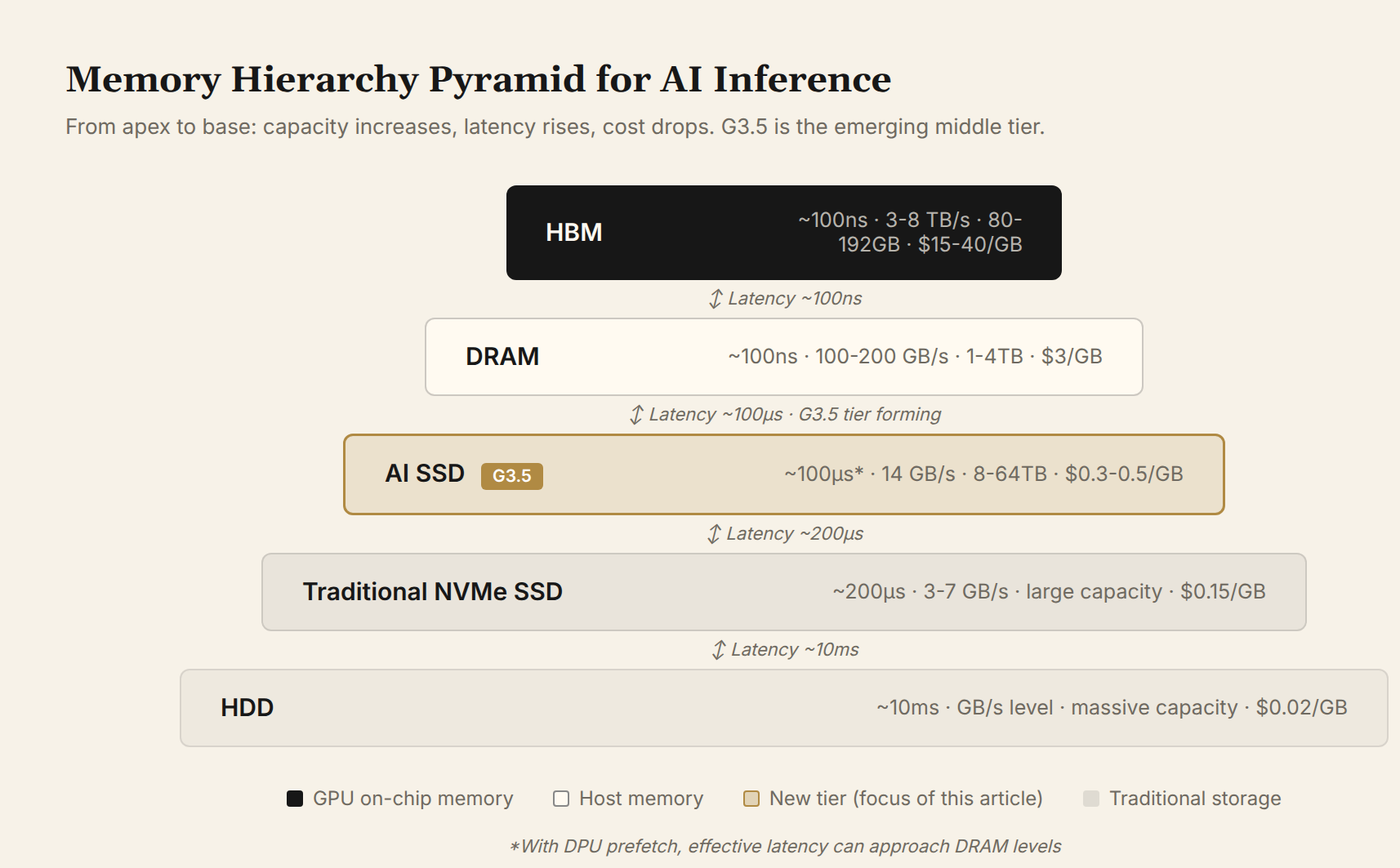
Figure 1: The memory hierarchy pyramid for AI inference. From apex to base, capacity increases, latency rises, and cost drops. G3.5 is the emerging middle tier — one to two orders of magnitude cheaper than DRAM, three to five times faster than traditional NVMe.
At the apex is GPU HBM: ~100ns latency, 3–8 TB/s bandwidth, 80–288 GB capacity — the most expensive. Below it sits DRAM: comparable latency but an order of magnitude lower bandwidth, with capacities reaching 1–4 TB. Further down are NVMe SSDs and HDDs. The G3.5 tier is shown as a dashed line — it is precisely the new layer whose necessity Chapter 6 will argue.
Chapter 2: Model Architecture — A Compression History of Attention
The evolution of attention mechanisms is, in essence, a history of KV Cache compression. Each architectural advance alters n_kv_heads or d_head in the formula from the previous chapter — or even changes the very organization of KV Cache itself.
| Architecture | Representative Models | KV Cache Compression Mechanism | Per-layer Per-token Size | Relative to GQA |
|---|---|---|---|---|
| MHA | Llama-2, GPT-3 | No compression; independent K/V per head | 2 × n_heads × d_head × 2B | ~2-4× |
| GQA | Llama-3, GLM, Qwen | Multiple query heads share one K/V group | 2 × n_kv_groups × d_head × 2B | 1× (baseline) |
| MLA | DeepSeek V3 | Joint K/V compression into low-dimensional latent variable | (d_latent + d_rope) × 2B | ~28% |
| Hybrid Compression | DeepSeek V4 | Sequence-dimension compression + sparse retrieval + sliding window | ~10 KB (full model) | ~3% |
MHA → GQA: Cutting KV Head Count
MHA (Multi-Head Attention) is the original scheme. For a ~70B model, 64 attention heads each have independent K and V matrices. Per-layer per-token KV Cache is 2 × 64 × 128 × 2 = 32 KB.
GQA (Grouped-Query Attention) takes a direct approach: keep 64 query heads, but reduce KV heads to 8 groups. Every 8 query heads share one K/V pair. Llama-3-70B uses this scheme. Per-layer per-token KV Cache drops to 2 × 8 × 128 × 2 = 4 KB — 12.5% of MHA.
The trade-off is reduced attention "resolution." 8 KV head groups serve 64 query heads; different query heads within the same group compute attention over the same K/V, theoretically reducing expressiveness compared to MHA where every head has its own K/V. However, extensive experiments show minimal quality degradation — under 1% on mainstream benchmarks. That trade buys an 8× KV Cache compression.
GQA is a one-time architectural decision made at training time. Existing models cannot be retroactively "upgraded" to GQA. And once you compress to 8 groups, pushing further (4 groups, 2 groups) accelerates quality loss. GQA's dividends are largely exhausted at the 8–16 group range.
At 1M context, GQA's limitations surface quickly. Llama-3-70B's GQA architecture produces 320 GB of KV Cache for a single 1M-context request — 4.6× the model weights. GLM-5.2 is worse: ~343 GB of KV per request, 2.0× the weights. Both numbers mean that under GQA at 1M context, holding a single request's KV Cache requires 2–3 eight-GPU H100 nodes.
GQA → MLA: Changing the Representation Space
DeepSeek V3's MLA (Multi-head Latent Attention) takes a fundamentally different path. GQA reduces the number of KV heads. MLA changes the representation space of K/V entirely.
Here is how MLA works. Instead of storing complete K and V vectors for each KV head, MLA jointly compresses K/V information into a low-dimensional latent vector c_kv (512 dimensions), plus a decoupled RoPE key (64 dimensions). At inference time, only (512 + 64) × 2 = 1,152 bytes/layer/token need to be cached — not separate K and V copies. When attention computation is needed, up-projection matrices W_up (512 → 128 heads × 128 dim) reconstruct the full K and V.
Per-layer per-token KV Cache drops from GQA's 4,096 bytes to MLA's 1,152 bytes — 28% of GQA. Across 61 layers, DeepSeek V3's per-token KV Cache is approximately 68.6 KB, and 1M context totals ~72 GB.
The cost is additional matrix multiplications for up-projection. Each layer has two up-projection matrices (recovering K and V respectively), with dimensions 512 × (128 × 128) = 8.4M parameters, roughly 32 MB/layer in weights. But these weights are fixed and shared across all tokens in a batch. The marginal compute overhead is under 5% of the attention itself. 5% more compute for 3.6× GQA memory compression.
MLA's deeper significance lies in decoupling "what to cache" from "what to compute." GQA reduces along the head dimension: fewer KV heads means narrower attention computation paths. MLA preserves the full attention computation path (128 heads × 128 dimensions, as wide as MHA) and compresses only the cached content. This insight paved the way for V4's hybrid compression: shifting the compression focus from the head dimension to the sequence dimension.
MLA → V4 Hybrid Compression: Compressing the Time Series
DeepSeek V4's hybrid compressed attention extends compression from the spatial dimension (heads) to the temporal dimension (sequence). V4 abandons V3's MLA in favor of a four-stage hybrid stack — not an incremental improvement over MLA, but an entirely new architecture.
KV Sharing (2× savings). All attention heads share the same Key and Value vectors. To preserve correctness, V4 applies an inverse RoPE operation at the attention output to recover positional encoding differences across heads. After sharing, the head dimension of KV Cache goes from "per-head" to "all-shared," immediately halving the footprint.
c4a Sequence Compression (4× savings). Along the sequence dimension, every 8 adjacent tokens have their KV vectors weighted-summed into 1 entry, with a stride of 4 (50% overlap between adjacent compression windows). The effect is a 4× reduction in sequence length. c4a handles fine-grained retrieval — not every token needs an independent K/V representation; neighboring tokens can share a compressed entry.
c128a Sequence Compression (128× savings). More aggressive: every 128 adjacent tokens are compressed into 1 entry. 128 tokens roughly equals one paragraph — a single entry is sufficient to maintain global semantic coherence. c128a handles coarse-grained global context.
DSA Top-K Sparse Selection. Even after c4a compresses the sequence to 1/4, 1M tokens still produce 250K compressed entries. Running full attention over all of them is too expensive. DeepSeek Sparse Attention selects the Top-1024 entries for attention computation. This reduces attention complexity from O(n²) to O(n×1024), cutting computation by two orders of magnitude at 1M context.
SWA Sliding Window (fixed 128 tokens). The most recent 128 tokens retain full-precision attention with no compression. Natural locality of language means the most recent few sentences have the tightest correlations — this segment cannot afford precision loss.
Of V4's 61 layers, 30 use CSA (Compressed Sparse Attention, with MLA components + Lightning Indexer) and 31 use HCA (Hybrid Compressed Attention, mixing c4a/c128a/SWA). The two layer types alternate. Different mechanisms serve different roles: SWA handles full-precision attention for the latest 128 tokens, c4a handles mid-range sparse retrieval, c128a handles long-range global compression, and DSA decides within each layer which entries are worth attending to.
The vLLM team verified the real-world impact on V4's release day: under BF16, V4-Pro's KV Cache for a single 1M-context request is only 9.62 GiB. Compared to the estimated 83.9 GiB for an equivalent-scale V3.2 GQA scheme, that is an 8.7× compression. With FP8 for attention cache and FP4 for indexer cache, KV Cache drops further to approximately 4.8 GiB.
Full Landscape: 1M Context Across Architectures
| Model | Attention Mechanism | KV/token (FP16) | Single-Request 1M KV | Model Weights | KV/Weight Ratio | 1M Feasibility |
|---|---|---|---|---|---|---|
| Llama-3 70B | GQA (8 heads) | 320 KB | 320 GB | 70 GB | 4.6× | ❌ |
| GLM-5.2 (est.) | GQA | ~328 KB | ~343 GB | ~170 GB | 2.0× | ❌ |
| DeepSeek-V3 671B | MLA | 68.6 KB | 72 GB | 671 GB | 0.11× | ⚠️ Marginal |
| DeepSeek V4-Pro | Hybrid Compression | ~10 KB | 9.62 GB | ~800 GB | 0.01× | ✅ Native |
The core message of this table: the KV/weight ratio drops from GQA's 2–4.6× to V4 hybrid compression's 0.01× — a 200× difference. At 1M context, GQA's KV Cache is the primary consumer of GPU memory (larger than the model weights). V4's KV Cache is almost negligible (1% of weights). This isn't about parameter tuning — it's a consequence of model design philosophy.
The architecture layer compresses each KV Cache from 320 GB to 9.62 GB, solving "how big is each one." But compression does not reduce the number of users — "how many are there total" is a question for the subsequent layers.
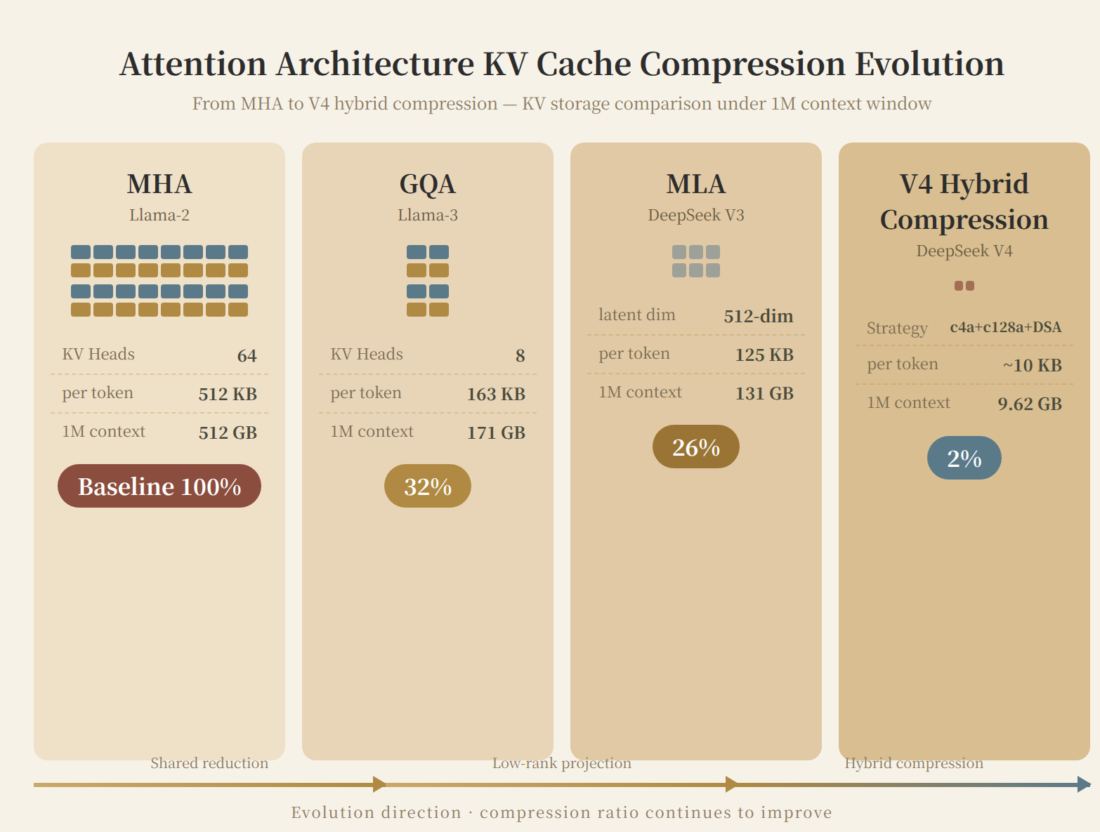
Figure 5: KV Cache compression evolution across attention architectures. From MHA's 512 KB/token to V4 hybrid compression's ~10 KB/token, per-request KV at 1M context drops from 512 GB to 9.62 GB.
Chapter 3: Precision and Encoding — 2-4× Instant Gains
Without changing model architecture, you can save GPU memory by lowering the storage precision of KV Cache. The gains are instant — a single config parameter — but the ceiling is clear: 2-4×.
The Precision Ladder
| Precision Mode | Relative Size | Quality Impact | Engineering Cost | Applicable Scenario |
|---|---|---|---|---|
| BF16/FP16 | 1× | Baseline | — | Offline, high-quality requirements |
| FP8 | 0.5× | Minimal (<1% quality loss) | Very low (vLLM --kv-cache-dtype fp8) |
General recommendation |
| INT4 | 0.25× | Moderate (requires calibration data) | Medium (calibration + validation) | Batch jobs, short context |
| FP4 Indexer (V4) | Additional ~2× (indexer portion) | Only affects indexer precision | Low (V4-specific parameter) | V4 only |
FP8 is the current engineering sweet spot. Nearly every modern inference engine (vLLM, SGLang, TensorRT-LLM) supports FP8 KV Cache by default. Quality loss has been tested across diverse tasks — under 1%, imperceptible in long-context generation. The cost of enabling it is one CLI argument: --kv-cache-dtype fp8.
DeepSeek V4 has an additional precision option: FP4 indexer cache. V4's CSA layers include a Lightning Indexer component used for DSA's Top-K selection. The indexer's KV Cache is stored in FP4, which does not affect main attention precision but further saves the indexer portion's memory. vLLM parameter: --attention_config.use_fp4_indexer_cache=True. Combined with FP8 attention cache + FP4 indexer cache, V4's KV Cache drops from BF16's 9.62 GiB to approximately 4.8 GiB.
INT4 quantization is more aggressive, compressing KV Cache to 1/4 of FP16. The problem is that quantization error accumulates over ultra-long contexts. The last 1% of tokens may exhibit noticeable deviation from accumulated quantization noise. INT4 requires calibration data, and calibration parameters are not transferable across different models and tasks. Currently, INT4 KV Cache is only suitable for quality-insensitive batch jobs or short-context scenarios.
Risks
KV quantization precision loss is amplified at ultra-long contexts. The reason is straightforward: during decode, each step reads the full KV Cache for attention, and quantization error propagates through every layer. Below 128K context, FP8 error is essentially invisible. But in the 512K–1M range, FP8's cumulative bias begins to surface in long-range dependency recall — the model occasionally "forgets" details mentioned very early. This loss is nearly imperceptible for coding assistants (code context typically stays within 128K), but for legal document analysis, cross-document reasoning, and other ultra-long-context scenarios, validation is needed.
Practical deployment recommendation: FP8 as the default baseline, enabled in all scenarios. INT4 only when memory is critically tight and the task tolerates precision degradation. FP4 indexer enabled per V4's official guidance.
The precision layer's gains are deterministic and zero-cost: 2-4×, from a single config parameter. For a model like V4 where KV Cache is already tiny, FP8 compresses 9.62 GiB to 4.8 GiB, letting a single GPU serve twice as many concurrent 1M requests.
Chapter 4: Inference Engines — Squeezing Every Byte
Model architecture determines how big each KV Cache is. The inference engine determines how that data is organized and used. The engine layer makes existing memory work smarter — the physical memory total stays the same, but effective capacity can increase 3-5×.
PagedAttention: Turning Memory Fragments into Blocks
In 2023, the vLLM team uncovered an embarrassing reality: traditional inference frameworks achieved only 30-40% GPU memory utilization. On an 80 GB H100, only 24-32 GB of KV Cache data was actually doing work. The remaining 48 GB was wasted to fragmentation and over-provisioning.
The root cause was memory allocation. Traditional frameworks pre-allocate a large contiguous KV Cache block per request, sized for the maximum possible context length. A request that ultimately uses only 4K tokens still holds a 32K reservation; the 28K of idle space cannot be shared. After the request finishes, the freed space may not be contiguous — like a parking lot with scattered empty spots, but no room to park a truck.
vLLM's PagedAttention borrows from operating system virtual memory paging. KV Cache is divided into fixed-size blocks, managed via a block table that maps logical to physical addresses. Each request gets exactly the blocks it needs, with no requirement for physical contiguity. Fragmentation waste drops from 60-80% to under 4%.
Block size is a critical tuning parameter. Too large (256 tokens/block), and small requests waste tail space. Too small (1 token/block), and the block table's own memory and lookup overhead climbs. vLLM's empirical sweet spot for traditional models is 16 tokens/block. DeepSeek V4 is special: c4a/c128a/SWA's three compression ratios mean different layers have different physical block sizes. vLLM's solution unifies on a 256-token logical block, with three compression ratios mapping to three physical page-size buckets, managed by a single allocator across three pools. This is a V4-specific engineering challenge, but transparent to the user.
Continuous Batching
Traditional static batching has an efficiency problem: requests within a batch have varying lengths. Short ones finish first, but GPU resources remain occupied by the long ones, and new requests cannot be inserted in time. Continuous batching schedules at the iteration level: after generating each token, the system checks for completed requests and immediately evicts them, then inserts waiting requests. GPU utilization jumps from 30% to over 70%. All modern inference engines now include this.
Prefix Caching: The Multi-Turn Force Multiplier
When multiple requests share a common prefix (system prompt, document context), each request redundantly recomputes the same KV Cache. Prefix caching stores these shared prefix KV Cache entries; new requests that hit the cache reuse them directly.
Hit rates vary dramatically across scenarios:
| Scenario | Typical Hit Rate | Savings |
|---|---|---|
| API service (shared system prompt) | 30-50% | Moderate |
| Coding assistant (multi-turn dialogue) | 85-95% | Enormous |
| Document RAG (multi-turn follow-up) | 80-90% | Enormous |
| One-shot long document analysis | 0% | None |
Why is the coding assistant hit rate so high? Consider a real workflow: Turn 1 sends [system: 8K] [file_context: 40K] [user: 0.5K], triggering prefill of 48.5K tokens. Turn 2 sends [system: 8K] [file_context: 40K] [turn1: 3K] [user: 0.5K], where 48.5K is reused from the previous turn — only 3.5K is new. Prefix Cache hits, skipping the redundant 48.5K prefill computation.
SGLang's RadixAttention implements prefix reuse as a Radix Tree. Each node represents a token sequence segment; the path from root to leaf is a request's complete context. Two requests sharing a prefix share a path in the tree, diverging at the point where they differ. Lookup and insertion are O(L) complexity (L = sequence length), essentially zero overhead. In Agent multi-turn dialogue scenarios (each turn shares all prior history), prefill computation from turn 2 onward drops by 80-95%.
These engine-layer optimizations compound, pushing effective memory utilization from 30% to over 90%. The same set of GPUs can serve 3-5× more users. But the physical memory total has not changed — rearranging shelves to reduce aisle waste lets you fit 30% more inventory, but the warehouse itself has not grown. To expand the warehouse, KV Cache needs to cross node boundaries.
Chapter 5: Cluster Architecture — Letting KV Cache Flow Across Nodes
Up to this point, KV Cache remains locked inside individual GPU HBM. The most active frontier in 2026 is liberating it into a cluster-level shared resource.
NVIDIA CMX: Moving KV Cache Out of the GPU
At CES in January 2026, NVIDIA announced CMX (Context Memory eXtension). The motivation is an engineering reality: in POD-scale inference clusters, many GPUs each store duplicate copies of the same KV Cache. An Agent application involving 20 dialogue turns needs each turn's KV Cache accessible on the GPU currently running inference. Multiple users querying the same Agent? The same system prompt's KV Cache is replicated N times.
CMX's core idea is to use a BlueField-4 DPU (Data Processing Unit) as an intelligent bridge between GPU HBM and external storage, centralizing these redundant KV Cache copies under unified management.
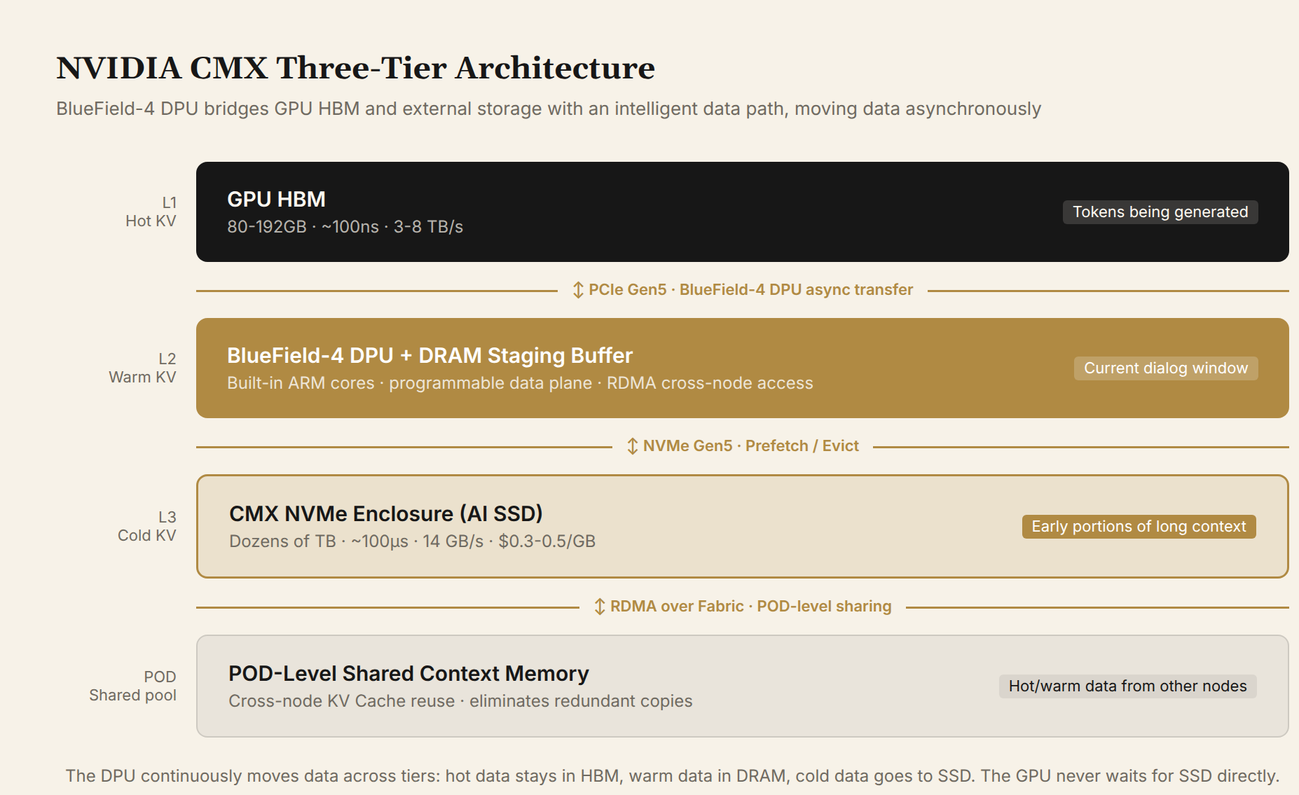
Figure 2: NVIDIA CMX architecture. The BlueField-4 DPU asynchronously moves data between each tier. Hot KV Cache stays in HBM; warm KV Cache sits in the DPU-attached DRAM staging buffer; cold KV Cache lands on AI SSDs in the CMX NVMe Enclosure. The GPU never directly waits for SSD reads.
The BlueField-4 DPU has built-in ARM cores and a programmable data plane, enabling cross-node data transfers without CPU involvement. Through RDMA, all GPUs in a POD can access the same context memory tier. This is especially significant for Agent inference: an agent accumulates long-range memory across multi-turn dialogue. Under traditional architecture, every participating GPU stores its own copy — 10 nodes means 10 redundant copies. Under CMX, that memory lives in a shared pool. Whichever GPU currently needs it reads it on demand. Redundancy eliminated.
NVIDIA Dynamo: Prefill-Decode Disaggregation
NVIDIA Dynamo is their open-source distributed inference framework, reaching 1.0 in early 2026. The key design is Prefill-Decode disaggregation.
Why separate the two phases? Because their hardware load profiles are polar opposites:
- Prefill is compute-bound. Processing 100K tokens of input requires 100K attention computations. GPU FLOPS saturate; each token's KV Cache is written once. The bottleneck is FLOPS.
- Decode is memory-bound. Each generated token requires reading all prior tokens' KV Cache for attention, but the computation is just one attention layer. The bottleneck is memory bandwidth.
Running both on the same node creates resource contention. When prefill saturates compute, decode starves. When decode saturates bandwidth, prefill's matrix multiplies cannot feed the GPU. Splitting them allows prefill clusters to use high-compute GPUs (like B300) and decode clusters to use large-HBM, high-bandwidth configurations. KV Cache passes between them through a shared storage pool: prefill nodes write KV Cache to the pool, decode nodes read from it.
For V4-Pro, Prefill-Decode disaggregation is especially rewarding. V4's hybrid compressed attention makes per-request KV Cache only 4.8 GB (FP8+FP4). Migrating a complete request's KV Cache across nodes over RDMA takes under 50ms — far below prefill's own computation time. This makes large-scale disaggregated deployment engineering-feasible.
Open-Source KV Cache Middleware: Four Projects
KV Cache disaggregation is not just an NVIDIA hardware play. Between 2024 and 2026, the open-source community produced multiple dedicated KV Cache middleware projects, each representing a distinct technical approach.
Mooncake (Moonshot AI / Kimi). The most complete centralized KV Cache disaggregation architecture to date, published at FAST 2025. Three components: KVCache Store (a distributed cache service deployed on inference nodes' idle CPU/DRAM/SSD), Transfer Engine (RDMA-based cross-node KV transfer, already integrated by vLLM, SGLang, and TensorRT-LLM), and Conductor (a global scheduler that selects prefill and decode instances based on KV Cache distribution). Published results: throughput improvement up to 525% in overload scenarios, and 75% more requests handled in Kimi's production environment. The core innovation: treating KV Cache as a first-class citizen for scheduling — not an inference engine appendage, but a distributed resource with its own lifecycle that can flow across nodes.
LMCache (UC Berkeley). Takes the "compatibility layer" route — no inference engine code changes, plugs in as a vLLM plugin. Multi-tier offload hierarchy: HBM → CPU DRAM → local SSD → remote storage, with LRU eviction. Backends are pluggable: local SSD, Redis, GPU Direct Storage, InfiniStore, Mooncake Store. In March 2026, LMCache was officially integrated into NVIDIA Dynamo as the KV caching layer solution. Public benchmarks show maximum servable context length increased 4-8× without affecting generation quality.
FlexKV (Tencent + NVIDIA). Released in January 2026, supports distributed KV Cache reuse based on Mooncake Transfer Engine. While LMCache focuses on single-node multi-tier caching, FlexKV targets cluster-level cross-instance reuse — multiple vLLM instances can share a single FlexKV backend, avoiding each instance independently caching identical KV.
NVIDIA Dynamo KVBM. The KV Block Manager in Dynamo 1.0, providing a three-layer architecture: LLM runtime → logical block management → NIXL transport, supporting both CPU and disk caching. Natively integrated with Dynamo's KV-aware routing — the scheduler knows which KV Cache blocks reside on which nodes and preferentially routes requests to nodes with existing cache.
Comparing the four projects' technical approaches:
| Project | Source | Core Innovation | Storage Backend | Integration Ecosystem |
|---|---|---|---|---|
| Mooncake | Moonshot AI | KVCache-as-a-service + Conductor global scheduling | DRAM + SSD (distributed) | vLLM, SGLang, TensorRT-LLM |
| LMCache | UC Berkeley | Multi-tier offload + pluggable backends | DRAM → SSD → Redis → Mooncake | vLLM, Dynamo |
| FlexKV | Tencent + NVIDIA | Cross-instance KV reuse | Distributed KV Store | vLLM, Mooncake Transfer Engine |
| Dynamo KVBM | NVIDIA | KV-aware routing + NIXL transport | CPU + disk | Dynamo native |
These projects are converging rather than competing. LMCache can use Mooncake Store as a backend. FlexKV uses Mooncake Transfer Engine for transport. Dynamo integrates both LMCache and KVBM. End users do not choose one of four — they combine these components on top of vLLM or SGLang.
On the commercial side, Huawei's UCM (Unified Context Memory) / CMS (Context Memory Service) solution is more aggressive. Huawei's published data shows TTFT (Time To First Token) reduced by 90% under PB-scale shared KV pool configuration. Huawei's advantage is a fully vertically integrated stack: from Ascend GPU to SSD controller, they own every layer.
Deep Dive: What Makes Up a Standalone KV Cache System?
The previous section surveyed four open-source projects and two commercial approaches. Making a technology selection requires a more structured framework. A standalone KV Cache system is not a single component — it is a combination of four foundational technologies: Transfer, Storage, Scheduling, and Integration. Each has independent technical challenges and clear divergences in approach.
Foundational Technology 1: Transfer Layer
The problem the transfer layer solves: how to move KV Cache between GPU HBM, CPU DRAM, SSD, and remote nodes with low latency, high bandwidth, and without blocking GPU computation.
Three mainstream transfer approaches exist today. RDMA (Remote Direct Memory Access) over InfiniBand or RoCE delivers 1–5μs latency and up to 400 Gbps bandwidth, making it the first choice for cross-node KV Cache migration. NVLink/NVSwitch uses NVIDIA's GPU interconnect with sub-μs latency, but only works within a single node. PCIe 5.0 + GPU Direct Storage lets GPUs bypass the CPU to read/write NVMe directly at 5–10μs latency, providing a direct GPU-to-SSD path.
At the architectural abstraction level, there are two design philosophies. One is generic data movement: NVIDIA's NIXL (NVIDIA Inference Transfer Library) does not care what the data is — it provides a unified API for frameworks to move data between storage tiers: GPU HBM → CPU DRAM → local NVMe → remote RDMA. NIXL is adopted by NVIDIA Dynamo as its underlying transport and can be independently used by vLLM. The other is KV Cache semantic binding: Mooncake Transfer Engine's API operates in block units that the inference engine understands, not byte-level copies. The migration unit is a KV block (typically corresponding to several tokens), and the transfer layer knows which block belongs to which request, which layer, which shard. This semantic binding lets the upper-layer scheduler simply say "transfer request A's KV Cache to node B" without worrying about how to chunk it at the bottom. The two paths are converging — Mooncake's upper-layer scheduling can invoke NIXL as its underlying transport.
There are three key technical challenges. Tail latency: RDMA's median latency is 2μs, but P99 can reach 50–100μs (network congestion, switch buffer overflow). In a Prefill-Decode disaggregated architecture, if a KV Cache migration stalls at P99, the decode node's GPU stalls. The solution is batch transfer + streaming migration: transfer layer by layer and start decoding progressively, using pipelining to hide latency. Mooncake's Conductor natively supports this inter-layer pipeline. Memory registration overhead: RDMA requires that memory be pre-registered (pinned to physical pages). Registering large blocks of KV Cache itself consumes CPU and time. NIXL mitigates this with on-demand registration + memory pool pre-warming. Multi-path load balancing: A single RDMA connection's bandwidth is limited (100–400 Gbps); large clusters need multi-path concurrency. Emerging solutions like UCCL P2P use collective APIs to automatically assign paths.
Evaluation criteria for a well-implemented transfer layer: (1) P99 latency no more than 10× the median; (2) per-node effective bandwidth reaching 80%+ of theoretical network bandwidth; (3) GPU utilization unaffected by transfers (transfer and computation overlap); (4) topology awareness — knowing which nodes are in the same NVLink domain and which require switch routing.
Foundational Technology 2: Storage Layer
The problem the storage layer solves: how KV Cache is stored, indexed, evicted, and kept consistent across different media (HBM/DRAM/SSD/distributed storage). It determines the cluster's total effective capacity and cross-tier hit rate.
The core is a three-tier storage hierarchy: GPU HBM as L1 (fastest, smallest, most expensive), CPU DRAM as L2 (comparable latency to HBM but an order of magnitude lower bandwidth), and SSD/distributed storage as L3 (large capacity, low cost, high latency). The key architectural abstraction: each tier exposes a unified block interface to the layer above, while internally implementing its own eviction policy and prefetch logic.
LMCache's implementation is the most representative. It plugs into vLLM without modifying inference engine code, providing HBM → CPU DRAM → local SSD → remote storage multi-tier offload. Between each tier, LRU eviction applies — frequently accessed KV Cache blocks automatically promote to faster tiers. Backends are pluggable: local SSD, Redis, GPU Direct Storage, InfiniStore, Mooncake Store. In April 2026, LMCache released a new architecture introducing In-Process Offload mode and Unified KV mode: the former performs KV Cache offload within the inference process, avoiding cross-process communication; the latter unifies KV Cache management across multiple GPUs, achieving 13.6× TTFT reduction on MoE models in testing.
SGLang's HiCache takes another approach. It extends RadixAttention from GPU memory to a three-tier hierarchy: GPU HBM is L1, host memory is L2, and distributed storage (such as Mooncake Store) is L3. Inspired by CPU's three-level cache: L1/L2 are private to each GPU, L3 is shared across nodes. HiCache uses a HiRadixTree to track where each node's KV Cache resides — GPU, CPU, remote storage, or multiple tiers simultaneously. When GPU memory fills up, HiCache automatically demotes blocks to CPU, then to Mooncake — all transparent to the inference engine.
There are four key technical challenges. Cross-tier hit rate: When a block is demoted from GPU to CPU and another request happens to need it, it must be reloaded. If the hit rate drops below 90%, effective latency reverts to the physical medium level, and inference performance degrades significantly. The key to improving hit rates is prefetching algorithms — expanded in Chapter 6. Eviction consistency: In a multi-tier cache, the same block may simultaneously exist as copies in both GPU and CPU. If one copy is modified (e.g., decode appends a new token), the other copy becomes stale. This requires write-through or write-back strategies. LMCache uses write-back (deferred synchronization, performance-first). SGLang HiCache uses write-through (immediate synchronization, consistency-first). Memory overhead: Cache metadata (block tables, hashes, TTLs) itself consumes memory — at 10K-scale concurrency, this can reach GB levels. Distributed storage integration (the next focus).
Foundational Technology 3: Scheduler
The problem the scheduler solves: under multi-node, multi-request, multi-SLO constraints, deciding which node handles each request, where to fetch and place KV Cache, and how to pair prefill with decode. This is the most information-dense component in the entire system — all transfer layer and storage layer capabilities are ultimately translated into actual performance through the scheduler.
At the architectural abstraction level, there are two routes. Centralized global scheduling: Mooncake's Conductor is the most complete implementation. Each request goes through three steps. First, Conductor checks which prefill instances already have reusable KV Cache and transfers the reusable portions there. Second, the prefill instance completes computation layer by layer while streaming the output KV Cache to the selected decode instance. Third, the decode instance loads the KV Cache and joins continuous batching. Conductor's optimization goal is to maximize KV Cache reuse while satisfying both TTFT and TBT SLOs. Decentralized routing: NVIDIA Dynamo's KV-aware routing does not schedule centrally. Instead, each router knows which KV blocks are cached on its node. When a request arrives, the router preferentially selects a node that already has the cache; if no cache exists globally, it picks the least-loaded node. Decentralized routing is lighter than Conductor but lacks Conductor's global view for cross-node reuse.
There are three key technical challenges. Multi-objective optimization under SLO constraints: Maximizing throughput vs minimizing latency is a classic tension. Mooncake's paper offers a practical approximation — optimize prefill scheduling to maximize cache reuse (subject to TTFT SLO), optimize decode scheduling to maximize throughput (subject to TBT SLO), then connect the two via KV Cache migration. Load skew: Hot system prompts' KV Cache gets frequently reused, causing some nodes to overload while others sit idle. Dynamo mitigates this with KV-aware routing + dynamic migration. Scheduling latency itself: Conductor's scheduling decisions require querying the global KV Cache index; at 10K-scale concurrency, the scheduling overhead itself becomes non-trivial. Mooncake uses two-level scheduling (coarse-grained node selection + fine-grained instance selection) to keep scheduling overhead under 1ms.
Evaluation criteria for a well-implemented scheduler: (1) global KV Cache reuse rate >70% (meaning 70% of requests at least partially hit existing cache); (2) scheduling decision latency <1ms (not a significant contributor to TTFT); (3) cross-node load balance CV (coefficient of variation) <0.3.
Foundational Technology 4: Integration Layer
The problem the integration layer solves: how the KV Cache system interfaces with the inference engine — remaining transparent to the engine (no changes to inference logic) while minimizing overhead (no significant latency introduced).
Two integration paths exist today. The first is vLLM's KVConnector interface: it defines a standard connector protocol. Any KV Cache backend that implements save_kv()/load_kv() can plug in. LMCache, Mooncake Store, and FlexKV all integrate with vLLM through this interface. The second is SGLang's HiCache native integration: KV Cache management is built into the inference engine, requiring no external plugins, but only supports SGLang's own HiRadixTree.
The core architectural tension is flexibility vs performance. The vLLM connector interface uses cross-process communication; each save/load requires serialization and IPC calls, with per-operation overhead of 50–200μs. At 10K-scale concurrency, this overhead accumulates significantly. LMCache's April 2026 architecture update introduced In-Process Offload mode to address this — offload logic completes within the inference process, with zero IPC overhead. SGLang's native integration naturally avoids this issue (zero-copy) but locks into SGLang. In practice: if using the vLLM ecosystem, choose LMCache or Mooncake connector; if using SGLang, use HiCache; if mixing both, use Mooncake Transfer Engine as the shared transport layer.
There are two key technical challenges. Lifecycle synchronization: The inference engine produces new KV Cache at each decode step (the new token's K/V). The integration layer must synchronize these increments to external storage without blocking inference. Asynchronous writes are the standard approach, but write-failure rollback handling is required. Version compatibility: Inference engine upgrades may change KV Cache's internal layout (e.g., V4's hybrid compression introduces multiple block sizes). The integration layer must adapt accordingly. vLLM's connector interface mitigates this through a version negotiation mechanism.
Evaluation criteria for a well-implemented integration layer: (1) TTFT increase after integration does not exceed 5%; (2) hot-pluggable support (switching backends without stopping service); (3) inference engine upgrades require only connector adapter changes, not core inference logic modifications.
Technology Selection Summary
A complete KV Cache solution must answer four questions: how to move data (transfer layer), where to store it (storage layer), who schedules it (scheduling layer), and how to plug into the inference engine (integration layer). The current mainstream combinations:
| Solution | Transfer Layer | Storage Layer | Scheduling Layer | Integration Layer |
|---|---|---|---|---|
| Mooncake | Transfer Engine (RDMA) | DRAM+SSD distributed | Conductor global scheduling | vLLM/SGLang/TRT-LLM connector |
| LMCache | Pluggable (GDS/RDMA/local) | Multi-tier offload | LRU + optional prediction | vLLM plugin |
| SGLang HiCache | Built-in + Mooncake backend | HiRadixTree three-tier | RadixAttention hit rate | SGLang native |
| NVIDIA Dynamo | NIXL | KVBM (CPU+disk) | KV-aware routing | Dynamo native |
There is no single optimal solution — only scenario matching. Single node, low concurrency: vLLM's built-in PagedAttention + Prefix Cache suffices. Multi-node Agent multi-turn dialogue: SGLang HiCache + Mooncake backend. 1,000-GPU cluster with PD disaggregation: Dynamo + NIXL + Mooncake Store. China environment without HBM: Huawei UCM + specialized SSD. The core judgment: KV Cache system complexity should be proportional to cluster scale — over-engineering and under-engineering are equally harmful.
How Distributed Storage Integrates with KV Cache Components
Foundational Technology 2 mentioned that the L3 tier of KV Cache needs to land on distributed storage. But distributed storage systems (such as Ceph, WEKA, VAST, Huawei distributed file systems) were not designed for KV Cache scenarios — they were built for traditional data services (files, blocks, objects). Making the two work well together requires solving three interface problems.
Access interface matching. KV Cache components (LMCache, Mooncake Store) need block-level read/write: fixed-size blocks stored and retrieved, with no file system semantics involved. Traditional distributed storage provides POSIX file interfaces or S3 object interfaces, where every read/write goes through the file system layer at millisecond-level overhead. There are two solutions. Mooncake Store's approach is to use the local file system (ext4/xfs) + direct block device access, bypassing distributed file systems entirely — its "distributed" nature is achieved through the Transfer Engine moving data directly between nodes, not through a shared file system. LMCache's approach is pluggable backends: local SSD direct block device, Redis (in-memory key-value), GPU Direct Storage (bypassing CPU), etc., avoiding hard dependencies on any specific distributed storage. If distributed storage is required (e.g., WEKA NeuralMesh), verify that it supports GPU Direct Storage or RDMA direct access — otherwise file system overhead will consume the performance budget.
Bandwidth and capacity planning. When distributed storage serves KV Cache, the key metric is not IOPS (KV Cache is not a random small-block workload) but sustained sequential read bandwidth. Chapter 6's calculations show that a single storage node needs 28–42 GB/s of sustained bandwidth to support the prefetch pipeline. This means the storage cluster's aggregate bandwidth must match the inference cluster's prefetch demand. Rule of thumb: storage aggregate bandwidth ≥ total inference GPUs × per-GPU prefetch rate (approximately 1–3 GB/s).
Data lifecycle. KV Cache is temporary data, not persistent data. After an inference request completes, the corresponding KV Cache should be reclaimed. Traditional distributed storage assumes data is long-lived; its garbage collection (GC) trigger frequency and granularity are unsuitable for high-frequency temporary data. Mooncake Store handles this through LRU + TTL auto-expiration. LMCache uses LRU eviction. If using traditional distributed storage, you need to explicitly configure short TTLs (5–30 minutes) and frequent GC — otherwise temporary KV Cache will quickly fill the storage capacity.
DeepSeek 3FS: A distributed file system with native KV Cache support. 3FS (Fire-Flyer File System) is a self-developed distributed file system open-sourced by DeepSeek in 2025, with 10K+ GitHub stars. Its positioning is unique — a storage system that treats KV Cache as a first-class citizen from day one.
Three architectural features make 3FS particularly suited for KV Cache workloads. First, disaggregated architecture with locality-oblivious access: it aggregates the bandwidth of thousands of SSDs and hundreds of storage nodes, so applications never need to care about data placement. A 180-node cluster (each with 2×200Gbps IB + 16×14TB NVMe) achieved 6.6 TiB/s read throughput under stress test. Second, CRAQ strong consistency: Chain Replication with Apportioned Queries — no eventual-consistency ambiguity, a KV Cache block is either read at the latest version or a consistent snapshot. Third, native KVCache interface: 3FS includes a built-in KVCache module, not an external plugin. KV Cache reads go through the USRBIO API, bypassing FUSE and page cache, achieving peak read throughput of 40 GiB/s per node on a 400Gbps NIC.
3FS addresses the three interface problems as follows. For access interface, 3FS offers both POSIX file interface (for training checkpoints) and USRBIO API (for direct KVCache access), avoiding POSIX overhead. For bandwidth, 6.6 TiB/s aggregate read throughput on 180 nodes is sufficient for 10K+ concurrent KV Cache prefetching. For data lifecycle, 3FS-KV supports TTL-based auto-expiration so KV Cache blocks do not accumulate indefinitely.
3FS has limitations: it is deeply optimized for DeepSeek's own hardware (InfiniBand + high NVMe count) and model architecture (MLA/hybrid compression, naturally small KV Cache). Under GQA architecture + Ethernet, 3FS's advantages diminish — GQA's KV Cache is so large that even 40 GiB/s per-node read bandwidth gets saturated quickly under concurrent load. 3FS's broader value is validating a design philosophy: a distributed file system can natively support KV Cache as a first-class data type, rather than adapting general-purpose storage after the fact.
Inference Cluster Performance Tuning: Key Metrics and KV Cache Effectiveness Evaluation
After deploying a KV Cache solution, how do you know if it is working? You need a quantifiable metrics framework and a controlled comparison methodology.
Core Performance Metrics.
| Metric | Definition | Target | KV Cache Impact |
|---|---|---|---|
| TTFT (Time To First Token) | Time from user request to first token returned | <2s (8K context) / <10s (1M context) | Very high — Prefix Cache hits reduce prefill computation |
| TPOT (Time Per Output Token) | Per-token generation time during decode | 30–50ms | Medium — KV Cache read speed determines whether decode stalls |
| Throughput | Tokens processed per GPU per unit time | Higher is better | Very high — concurrency is limited by KV Cache capacity |
| Concurrency | Number of requests served simultaneously | Limited by total KV Cache budget | Directly determined |
| KV Cache Hit Rate | Prefix Cache or cross-request reuse hit rate | Coding assistant >85%, API service >50% | Directly measures Prefix Cache effectiveness |
| GPU Utilization | Fraction of time GPU spends computing | >70% | Indirect — engine optimizations improve utilization |
| Memory Utilization | Ratio of effective KV Cache data to allocated space | >90% | Directly measures PagedAttention effectiveness |
Pre- and Post-Deployment Comparison Testing Methodology.
The core principle of comparison testing: control variables. Change only the KV Cache configuration; keep everything else (model, hardware, workload) constant.
Step 1: Establish a baseline. Run a fixed set of workloads with the standard inference engine (e.g., vLLM default config, only PagedAttention enabled, no Prefix Cache / offload). Record the 7 metrics above. The workload should cover three scenarios: short context (8K), medium context (64K), and long context (256K), using either real request traces or synthetic data.
Step 2: Enable optimizations incrementally, one at a time. First enable FP8 KV Cache and measure; then enable Prefix Cache and measure; then add LMCache (CPU offload) and measure. Record metric changes at each step.
Step 3: Enable everything and run mixed workloads. Verify that the compounded effect matches expectations.
Key comparison metrics:
| Optimization | Expected TTFT Change | Expected Throughput Change | Expected Concurrency Change |
|---|---|---|---|
| FP8 KV Cache | No change | +80–100% | +100% |
| Prefix Cache (85% hit rate) | −60–80% | +20–50% | No change |
| CPU Offload (LMCache) | +5–10% | +10–30% | +50–200% |
| PD Disaggregation | −20–40% | +100–200% | +100–300% |
If actual improvements fall significantly below expectations (e.g., Prefix Cache hit rate shows 85% but TTFT only drops 20%), the bottleneck is not in KV Cache but elsewhere — possibly GPU compute (decode phase compute-bound), network bandwidth (cross-node transfer-bound), or engine scheduling overhead.
Bottleneck Identification Method.
When performance metrics fall short, troubleshoot in the following order:
- GPU compute bottleneck: Check GPU utilization. If >95% and throughput plateaus with increasing concurrency, compute is saturated. KV Cache optimization cannot help — add GPUs or upgrade to faster cards.
- Memory capacity bottleneck: Check OOM frequency. If increasing concurrency triggers OOM, KV Cache has filled GPU memory. Countermeasures: enable FP8, add CPU offload, or implement PD disaggregation.
- Bandwidth bottleneck: Check GPU utilization during decode. If decode-phase GPU utilization is very low (<30%) and TPOT is high, decode is waiting for KV Cache reads — memory-access bound. Countermeasures: ensure hot KV Cache is in HBM; check DPU prefetch hit rate.
- Network bottleneck: Check cross-node KV Cache migration latency. If TTFT increases after PD disaggregation, network migration latency exceeds the prefill computation savings. Countermeasures: increase RDMA bandwidth, use streaming migration.
- Scheduling bottleneck: Check request queuing time. If requests wait a long time after arrival before being scheduled, the scheduler is the bottleneck. Countermeasures: simplify scheduling logic or add scheduler instances.
This metrics framework and troubleshooting process should be a standard component of every inference cluster's operations documentation. No measurement means no optimization — KV Cache solution effectiveness must be validated with data, not judged by feel.
CXL: Another Path
CXL (Compute Express Link) is a low-latency interconnect standard that bypasses traditional PCIe. Its advantage is memory semantics: CPU/GPU access to remote CXL memory is identical to accessing local DRAM — no file system, no IO queues, no block device abstraction. Read/write requests go directly to the target address. Latency is in the 200-500ns range, two orders of magnitude faster than NVMe.
Marvell's Structera S 30260 is a CXL device specifically designed for cache expansion. However, CXL 3.0 deployments remain rare. CXL-compatible server motherboards, RCD chips, and memory controllers are still in early stages. CXL memory expansion modules are currently DRAM-based, with costs still at ~$3/GB. In the near term, the NVMe + DPU combination leads, thanks to its mature PCIe ecosystem and abundant off-the-shelf SSD products. CXL is more of a "next generation" solution, waiting for ecosystem maturation around 2027-2028.
Chapter 6: Storage Devices — When SSD Becomes Memory
The first five chapters traverse the complete optimization chain: architecture compression shrinks KV Cache to 3% of GQA; precision encoding halves it again; engines push memory utilization from 30% to 90%; cluster architecture lets KV Cache flow across nodes. The gap has narrowed dramatically — but it has not vanished. 100 concurrent 1M-context requests, even after V4-level compression and pooling, still require hundreds of GB of KV Cache space. What HBM and DRAM cannot hold must spill to the next tier.
KV Cache Is Not a Traditional Storage Workload
KV Cache read/write characteristics differ fundamentally from traditional storage (databases, file systems). The choice of storage medium is determined by access patterns.
Writes: The Prefill phase writes the entire context's KV Cache in one pass — large blocks, sequential, written once. A 100K-token prefill produces roughly 32 GB of data (70B GQA), after which only incremental per-token appends occur during decode (~320 KB/step). There is nothing like the small-block random writes of a traditional database.
Reads: The Decode phase reads the full cached KV Cache for attention at every step. But attention access distribution is extremely uneven. Multiple long-context attention distribution studies have found a consistent pattern: attention weights show strong local concentration, typically 70-90% focused on the most recent several K tokens. Remote context beyond 16K tokens is still accessed, but with low weight share (10-20%) and highly sparse access positions.
| Dimension | KV Cache Requirements | Traditional Database Workload |
|---|---|---|
| Writes | Large-block sequential, low frequency | Small-block random, high frequency |
| Reads | Batch, locally concentrated, prefetchable | Random, unpredictable |
| Capacity | 0.5-2 TB per node | 4-16 TB per node |
| Latency sensitivity | Effective latency must be < 10ms | Can tolerate 10-100ms |
Why SSD Effective Latency Can Approach DRAM
SSD physical access latency is ~100μs. DRAM is ~100ns. That is a 1,000× gap. Using SSD directly as memory would cripple inference. Yet in production deployments, SSD effective latency can approach DRAM. The answer is attention access patterns + DPU prefetch pipelining.
Hot data (70-90% of accesses) = KV Cache for the most recent several K tokens. For a 70B GQA model, 16K tokens of KV Cache is ~5 GB — easily held in HBM or DRAM at 100ns latency.
Cold data (10-20% of accesses) = all context preceding the hot window. 1M tokens minus 16K ≈ 1M tokens of KV Cache. This data is rarely accessed. Storing it on SSD does not affect inference speed.
The critical question: when attention does need to access cold data (that 10-20% of long-range dependencies), will SSD's 100μs latency cause GPU stalls?
This is where DPU prefetching comes into play. While the GPU is still processing the current token, the BlueField-4 DPU has already moved the next batch of cold KV blocks from SSD into the DRAM staging buffer. The prefetch strategy has three layers:
- Sliding window prefetching: Maintains a continuously moving hot data window (4-16K tokens ahead of the current decode position). KV Cache within this window is always kept in DRAM.
- Attention pattern prediction: For known attention patterns (e.g., early context repeatedly referenced in Agent multi-turn dialogue), the DPU proactively moves corresponding blocks to DRAM.
- Cross-request reuse: When multiple users share the same context segment, only one copy is prefetched to the shared pool.
Let's verify the prefetch math. Assume the DPU maintains a 4K-token prefetch window. For a 70B GQA model at 320 KB/token, the window totals 4,096 × 320 KB ≈ 1.3 GB. PCIe 5.0 NVMe sequential read bandwidth is 14 GB/s, so the transfer takes ~93ms. How long does decode take to consume those 4K tokens? At 10-30ms per token, 4K tokens take 40-120 seconds. The SSD has a 400-1,200× time headroom to complete the prefetch.
The DPU does not wait until the GPU needs data to read from SSD. It moves the next batch ahead of time while the GPU is still busy with the current token. By the time the GPU actually needs that data, it is already in DRAM. The effective latency the GPU sees approaches DRAM levels (~100ns), not SSD's physical latency (~100μs).
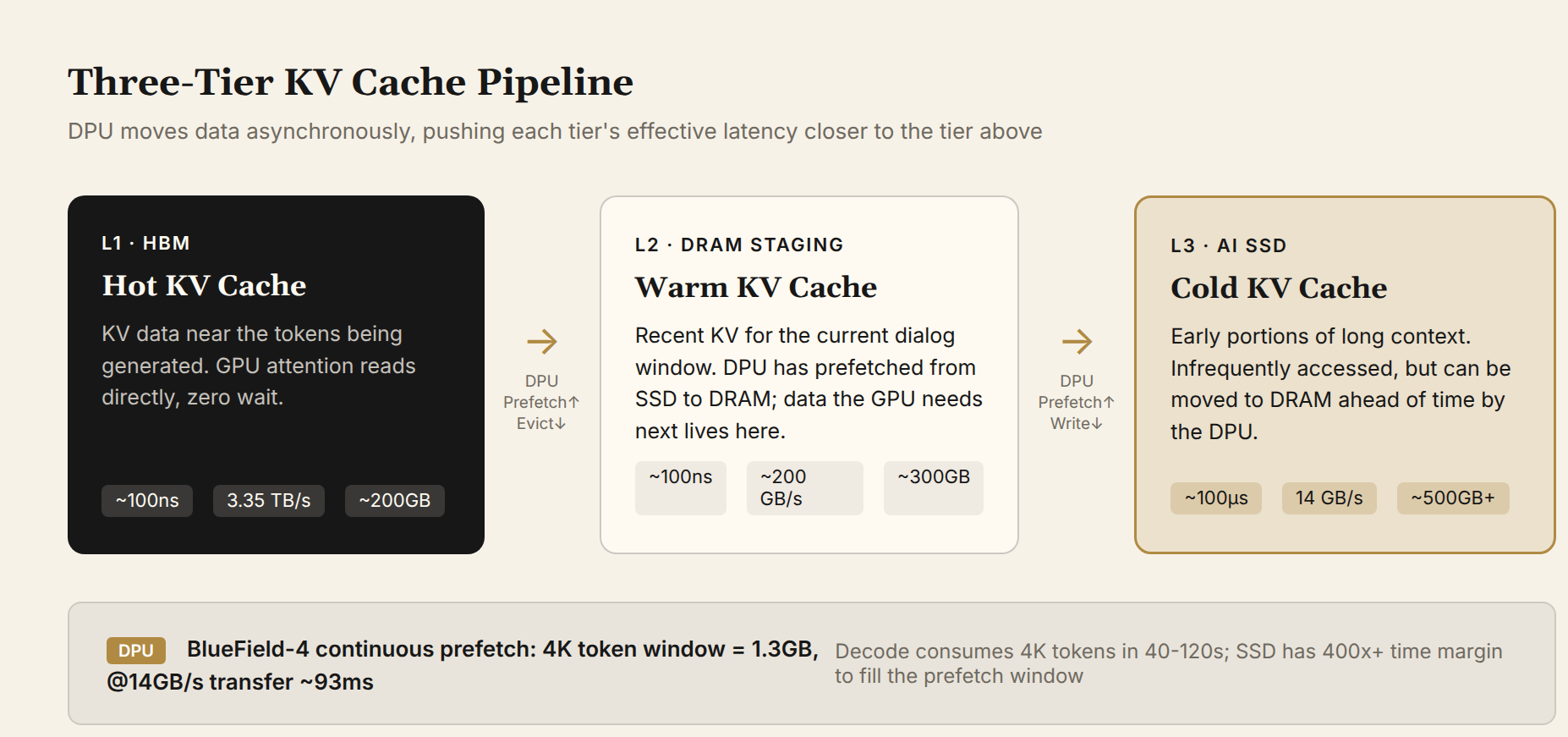
Figure 3: Three-tier KV Cache pipeline. The hottest KV Cache (current attention window) is in HBM; warm data (prefetch window) is in the DPU-attached DRAM staging buffer; cold data (earlier portions of long context) is on AI SSD. The DPU asynchronously moves data so that each tier's effective latency approaches the tier above.
NVIDIA's CMX architecture data presented at ICMSP 2026 shows that in 128K-context scenarios, DPU prefetch hit rate exceeds 90%. Accesses that miss and fall back to SSD physical latency are under 10%. This 10% miss penalty is partially absorbed by the attention computation's asynchronous pipeline, keeping GPU stall time within acceptable bounds. Getting from 90% to 95% requires three software-level breakthroughs: attention-pattern-based access prediction (beyond LRU), token-level prefetch granularity, and cross-request KV Cache reuse scheduling. All three are software problems — no new hardware needed. Estimated convergence: 12-18 months.
A New Category: AI SSD
When SSD's role shifts from "a warehouse that stores data" to "a memory extension layer that participates in computation," a new product category is forming.
Kioxia CM9 is an enterprise SSD supporting the CMX architecture protocol, with PCIe 5.0 interface and 14 GB/s sequential read bandwidth. Kioxia also introduced the GP Series (flash products connecting directly to GPUs) — the hardware that truly defines this new category. By bypassing traditional SSD controllers and interfacing directly with GPUs, it creates a low-latency flash layer. Kioxia has NAND production advantages (world's second largest) and no HBM business, meaning no self-cannibalization risk. If G3.5 becomes a real category, Kioxia is making the biggest bet.
Innogrit Dongting N3X pushes parameters more aggressively: 14 GB/s read, 3,500K IOPS, high endurance. It uses Kioxia XL-FLASH storage-class memory rather than standard NAND, keeping latency at one-third of traditional TLC SSD, with DWPD improved 30× over traditional enterprise SSDs. Traditional enterprise SSDs typically have DWPD of 1-3; a 30× improvement means these drives are designed for sustained large-block sequential writes typical of KV Cache scenarios — not the random writes of traditional databases.
Dapustor X5 focuses on FDP (Flexible Data Placement) plus transparent compression. FDP lets the SSD controller manage flash block allocation more efficiently, keeping write amplification under 1.5×. Transparent compression runs in real-time at the controller level; the repetitive attention patterns in KV Cache achieve respectable compression ratios, making effective usable capacity larger than nominal.
Solidigm D5 takes the QLC high-capacity route, with single-drive capacity reaching 60TB+, extremely low $/GB cost — suitable as the coldest tier in KV Cache layering.
Industry Landscape: Who's Aggressive, Who's Cautious
Samsung and Solidigm (SK Hynix + Intel NAND joint venture) are both on the ICMSP validation list, but neither has loudly launched an "AI SSD" category. The reason is not hard to guess: both have substantial HBM businesses. In 2025-2026, HBM production capacity is supply-constrained, with ASPs continuing to rise. Actively promoting the narrative of "using SSD to replace some HBM" means cannibalizing their most profitable product line.
Micron took a different path, focusing on CXL. CXL's memory-semantic access is inherently better suited for "use as memory" than NVMe, but the ecosystem needs more time to mature.
Chinese vendors are the most aggressive. Innogrit, Dapustor, plus Huawei's UCM solution, made a dense series of product and solution announcements at the CFMS|MemoryS 2026 summit. The reason is simple: Chinese vendors cannot procure advanced HBM. Export controls have narrowed the HBM acquisition channel severely. Chinese inference solutions (such as Huawei Ascend + UCM) never had HBM to begin with — SSD is the only massively available storage medium. G3.5 for them is not "replacing HBM"; it is "there was never HBM, SSD is the only option."
Cost Comparison: The Commercial Rationale for G3.5
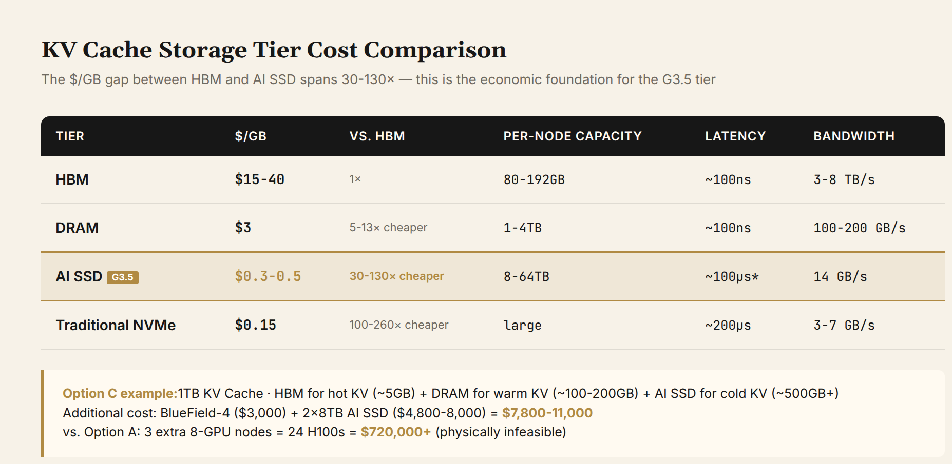
Figure 4: Cost and performance comparison across storage tiers. Note the 30-130× $/GB gap between HBM and AI SSD.
| Tier | $/GB | Relative to HBM | Per-Node Capacity | Latency | Bandwidth |
|---|---|---|---|---|---|
| HBM | $15-40 | 1× | 80-288 GB | ~100ns | 3-8 TB/s |
| DRAM | $3 | 5-13× cheaper | 1-4 TB | ~100ns | 100-200 GB/s |
| AI SSD (G3.5) | $0.3-0.5 | 30-130× cheaper | 8-64 TB | ~100μs* | 14 GB/s |
| Traditional NVMe SSD | $0.15 | 100-260× cheaper | Large | ~200μs | 3-7 GB/s |
*Effective latency with DPU prefetching can approach DRAM levels.
HBM costs $15-40 per GB. AI SSD costs $0.3-0.5 per GB — a 30 to 130× gap. For a scenario requiring 1 TB of KV Cache storage, using HBM requires the equivalent of ~13 H100 GPUs' worth of memory (at $30,000+ each). Using AI SSD requires $300-500 worth of drives. This cost gap is the commercial rationale for the G3.5 tier. It does not exist to replace HBM — it exists to absorb the KV Cache data that cannot fit in HBM but is too latency-sensitive for traditional storage.
Chapter 7: Cluster Economics and Decision Framework
A 1,000-GPU B300 × V4-Pro Cluster Case Study
Let us put all five optimization layers into a real cluster and run the numbers.
NVIDIA B300 (Blackwell Ultra) specs: 288 GB HBM3e, 8 TB/s bandwidth, 13.1 PF dense FP4, NVLink 5 bidirectional 1.8 TB/s, 1400W liquid cooling. A 1,000-GPU cluster = 125 eight-GPU nodes. Total HBM: 288 TB. Total FP4 compute: 13.1 EF.
DeepSeek V4-Pro weights load natively in FP4. Under expert parallelism (8-way), each GPU carries ~91 GB expert weights + 150 GB dense layer weights (fully replicated) + 5 GB embedding ≈ 155 GB. Runtime overhead: ~25 GB. Per-GPU available KV Cache budget:
288 GB (HBM) - 155 GB (weights) - 25 GB (runtime) = 108 GB
Conservatively: 110 GB
Single-GPU Concurrency Capacity
| Context | KV/Request (BF16) | KV/Request (FP8+FP4) | Concurrency (BF16) | Concurrency (FP8+FP4) |
|---|---|---|---|---|
| 32K | 0.30 GB | 0.15 GB | 333 | 666 |
| 128K | 1.20 GB | 0.60 GB | 83 | 166 |
| 256K | 2.41 GB | 1.20 GB | 41 | 83 |
| 512K | 4.81 GB | 2.40 GB | 20 | 41 |
| 1M | 9.62 GB | 4.80 GB | 10 | 20 |
The 1,000-GPU cluster (125 replicas) at 1M context with FP8+FP4 achieves total concurrency = 20 × 1,000 = 20,000 concurrent 1M-context requests.
Compare with GQA: the same 1,000 B300 GPUs running a GLM-5.2-class model (GQA, KV/request 343 GB) needs 343/110 ≈ 4 GPUs per single 1M request. 1,000 GPUs serve only 250 concurrent 1M requests — 80× worse.
Five-Layer Compounding Effect
From bare bones to fully optimized, V4-Pro's 1M-context KV Cache evolves as follows:
| Optimization Layer | Method | KV/Request | Cumulative Compression |
|---|---|---|---|
| Bare GQA equivalent | None | ~170 GB | 1× |
| + Architecture compression | V4 hybrid attention (BF16) | 9.62 GB | 18× |
| + Precision compression | FP8 + FP4 indexer | 4.80 GB | 35× |
| + Prefix Cache | 85% hit rate (amortized over multi-turn) | 0.72 GB | 236× |
| + Prefill-Decode disaggregation | Throughput +2-3× | — | ~500× effective |
Bare GQA @ 1M: 170 GB/request, 1,000 GPUs serve ~340 concurrent. V4 fully optimized @ 1M: ~0.7 GB/request (amortized), 1,000 GPUs serve ~157,000 effective concurrent.
This 460× gap is the compounding value of model architecture + inference engineering + cluster architecture.
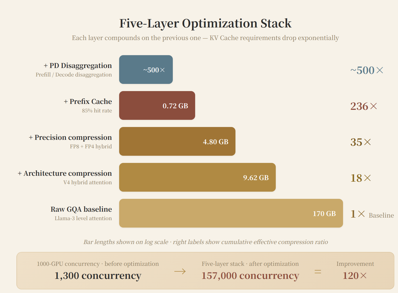
Figure 6: Five-layer optimization stack. From raw GQA's 170 GB/request to fully optimized ~0.7 GB/request (amortized), a 500× cumulative compression. The 1,000-GPU cluster's effective concurrency rises from 340 to 157,000.
Decision Framework: When to Do What
Is KV Cache acceleration mandatory or optional?
This question has a clear quantitative answer. The criterion: GPU savings from KV Cache optimization ≥ 1.5× the optimization cost. Beyond this inflection point, not optimizing is burning money.
The inflection point formula:
Inflection condition: N_concurrent × KV_per_token × S_avg ≥ 0.5 × W_model
When the total KV Cache across all concurrent requests reaches 50% of model weights, KV Cache optimization shifts from "optional" to "mandatory."
Take a 70B GQA model: weights 70 GB (FP8), KV/token 320 KB (FP16). 0.5 × 70 GB / 320 KB ≈ 215K tokens. That is, when the total token count across all concurrent requests exceeds 215K, you are past the inflection point. At an average context of 8K, 27 concurrent requests clears it. At 32K average context, just 7 concurrent requests do.
Specific inflection points by model and context:
| Model | Architecture | Weights (FP8) | KV/token | Inflection (concurrency, 32K context) | Inflection (concurrency, 128K context) |
|---|---|---|---|---|---|
| Llama-3 70B | GQA | 70 GB | 320 KB | 7 | 2 |
| DeepSeek V3 671B | MLA | 671 GB | 68.6 KB | 84 | 21 |
| DeepSeek V4-Pro 1.6T | Hybrid Compression | ~800 GB | ~10 KB | Far above practical concurrency | Far above practical concurrency |
| GLM-5.2 (est.) | GQA | ~170 GB | ~328 KB | 3 | 1 |
This table reveals several things. GQA architecture is past the inflection point in any real-world serving scenario — as long as someone is using it, optimization pays for itself. MLA architecture significantly delays the inflection point; benefits start at medium concurrency. V4 hybrid compression almost never hits the inflection point (KV is too small) unless concurrency is extreme.
Selecting Optimization Tiers by Cluster Size:
| Cluster Size | Must-Do | Recommended | Optional |
|---|---|---|---|
| 1-4 GPUs | PagedAttention | FP8 KV | — |
| 8-32 GPUs | + Prefix Cache | + Continuous Batching | INT4 exploration |
| 64-256 GPUs | + All of the above | + Prefill-Decode disaggregation | Cross-node KV pooling |
| 1,000+ GPUs | + All of the above | + KV pooling + elastic scheduling | MTP / custom kernels |
Assessing KV Cache Importance by Context Length:
| Context | KV/Weight Ratio (GQA) | KV Cache Role | Optimization Investment |
|---|---|---|---|
| < 8K | < 5% | Negligible | Default PagedAttention |
| 8-32K | 5-30% | Noticeable | FP8 + Prefix Cache |
| 32-128K | 30-100% | Important | Full engine optimization suite |
| 128K-512K | 100-500% | Core cost | + Disaggregated architecture + storage |
| 1M | 500%+ | Existential requirement | Must use architecture-compressed model |
Build vs API Inflection Point:
A 1,000-GPU B300 × V4-Pro cluster costs approximately $1.17M/month to operate. DeepSeek V4-Pro API output price is $0.87/M tokens. Break-even: $1.17M / $0.87 ≈ 1.34B output tokens/month, or ~45M output tokens/day. At an average of 10K output tokens/request, that is ~4,500 requests/day.
Above 5,000 daily requests (including ultra-long context), a self-built 1,000-GPU cluster is economically viable. Below 1,500, API is more cost-effective. The middle ground depends on utilization — an idle cluster burns ~$1,600/hour. Without stable demand, do not build.
The Real Bottleneck Has Moved Beyond Memory
For the V4-Pro + B300 combination, the 1,000-GPU cluster's bottleneck shifts away from memory:
| Dimension | Status | Notes |
|---|---|---|
| KV Cache memory | ✅ Abundant | 1M request uses only ~5 GB; 110 GB budget is more than enough |
| MoE all-to-all communication | ⚠️ True bottleneck | 49B activated parameters' expert routing needs NVLink-level bandwidth |
| Prefill compute | ⚠️ Bottleneck | 1M-token prefill is compute-bound; needs dense FP4 FLOPS |
| Decode latency | ✅ Good | V4's sparse attention makes decode nearly O(1) |
Inference optimization investment should pivot from "saving KV Cache" to "accelerating expert routing and long-context prefill."
Closing: The Bottleneck Has Moved
Returning to the opening contradiction: 320 GB of KV Cache demand, 80 GB of HBM — where does the difference go?
The five-layer optimization chain provides the answer. Architecture compression: 320 GB → 9.62 GB (18×). Precision encoding: 9.62 → 4.8 GB (35×). Inference engines push memory utilization from 30% to 90%+. Cluster architecture lets KV Cache flow across nodes, eliminating redundancy. Storage devices use AI SSDs at 1/100th the cost of HBM to absorb spilled cold data, with DPU prefetching making effective latency approach DRAM. Layer Prefix Caching on top for multi-turn scenarios, and effective KV footprint per request drops below 1 GB.
The optimization center of gravity has shifted from the inference system layer to the model architecture layer. In the GQA era, inference engineers tuned parameters in vLLM. In the V4 hybrid compression era, compression happens at model design time — the inference engineer's job becomes understanding the attention architecture and designing matching deployment topologies. The new bottlenecks are MoE communication, prefill compute, and DPU prefetch hit rates — the next frontier of inference optimization.
Risks remain. G3.5's effectiveness depends on DPU prefetch pipeline maturity. If scheduling algorithms are not good enough, SSD effective latency reverts to physical levels and inference performance degrades significantly. CMX, CXL, and open-source solutions — three competing standardization paths — have not yet converged.
But these uncertainties do not change one fundamental fact: model context windows have moved from 8K to 1M. Inference has moved from single-turn Q&A to Agent long-range memory. KV Cache growth is structural. HBM capacity growth is not. This structural divergence is the fundamental reason the entire optimization chain exists.
This article is based on publicly available information, including NVIDIA official releases (CES 2026, GTC 2026, ICMSP 2026), the CFMS|MemoryS 2026 industry summit, product announcements from Kioxia/Innogrit/Dapustor, vLLM technical blog posts, DeepSeek technical discussions, and arXiv papers. It does not constitute investment advice. Data is current as of June 15, 2026.