
GPU clusters have already exceeded the power supply limits of a single site. The next step—not building bigger, but connecting farther.
AI Clusters Are Growing a Third Dimension
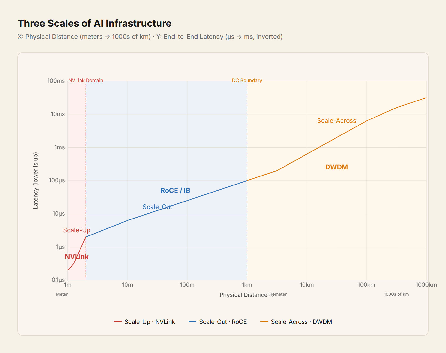
To understand Scale-Across, first take a look at the full coordinate system:
| Dimension | Physical Range | End-to-End Latency | Bandwidth | Transmission Medium | Parallel Strategy Supported |
|---|---|---|---|---|---|
| Scale-Up | Within rack (<2 m) | <1μs | TB/s | NVLink / UALink | Tensor Parallelism (TP) |
| Scale-Out | Single data center (<1 km) | 10-100μs | 400-800GbE | IB / RoCE | Pipeline Parallelism (PP), Data Parallelism (DP) |
| Scale-Across | Cross data center (50-2000 km) | 0.5-20ms | 100+ Tbps | Long-haul DWDM / Hollow-core Fiber | Async Data Parallelism, RL Training |
In the AI training networking space, most attention over the past two years has focused on the first two dimensions. For Scale-Up: NVLink supernode solutions (NVL72, Ascend 384). For Scale-Out: topology evolution (ZCube, RailFly, 3D Torus). But in July 2026, at least four signals appeared globally, all pointing to the third dimension transitioning from lab to engineering deployment. This article covers precisely that: why Scale-Across went from a "maybe possible" alternative to a "must-do" infrastructure architecture, who is doing it, and what technical gaps remain.
§1 What Is Scale-Across
Start with a mental image: 512 GPUs are 83 km away, and you want them to train a model together with another 512 GPUs in the primary cluster. A single AllReduce operation requires all 1024 GPUs to send gradients simultaneously and wait for aggregated results. Light traveling through optical fiber covers 83 km round trip in about 0.81 ms (2/3 of vacuum speed; hollow-core fiber would be faster). Adding forwarding equipment processing, the end-to-end delay is roughly 0.9 ms.
What does 0.9 ms mean? If we are waiting on AllReduce, those 1024 GPUs do nothing for the next ~1 ms—pure idle cycles. At 2 PFLOPS per H100, 1 ms of idling means roughly 2 TFLOPS of compute capacity is completely wasted in that 1 ms. For a training throughput of 3000 steps/second, every extra 1 ms per step consumes 3 seconds of GPU time per second. This does not even account for the cascading losses from packet retransmission—a 1‰ packet loss rate can cut training efficiency in half.
This scenario is the core problem Scale-Across aims to solve: connecting geographically dispersed data centers into a logical GPU cluster within the AI training backend network.
It differs fundamentally from traditional "Data Center Interconnect" (DCI). DCI carries frontend traffic (storage backup, data synchronization, cloud resource scheduling, inference request distribution), tolerating millisecond-level latency, with traffic patterns similar to traditional cloud networks. Scale-Across carries backend traffic—gradient synchronization during training (AllReduce, All-to-All)—which is part of GPU co-computation, and is extremely latency-sensitive with zero tolerance for packet loss.
This distinction matters because AI training traffic exhibits a unique pattern: synchronous bursts. An AllReduce operation sends gradients from all GPUs into the network within a few milliseconds simultaneously, creating an instantaneous spike of hundreds of thousands of concurrent flows hitting the switch. Traditional DCI shallow buffers (hundreds of KB to a few MB) collapse instantly under this pattern, packet loss skyrockets, and GPU idling is triggered. So Scale-Across is not as simple as "pulling a fiber-optic cable between two buildings." It requires simultaneous adaptation at the physical layer, link layer, transport layer, and training framework layer so that GPUs 83 km away feel "as if they were in the same rack."
§2 Why Scale-Across Suddenly Became Urgent
Start with a set of data points from mid-2026:
- Gartner's data center infrastructure forecast (2026.7.9): global data center total power consumption 132 GW, +27% YoY. AI-optimized server power growth rate at 84.2%, projected to exceed traditional servers by 2027
- US high-voltage generator transformer lead times are approaching 160 weeks (Wood Mackenzie, May 2026 report). About 52 weeks in 2020, 77 weeks in 2023, over 3 years in 2026. High-voltage circuit breaker lead times also extended from 77 weeks (2023) to 125 weeks
- Meta internal memo leaked (Reuters, 2026.7.9): deploying 7 GW of compute infrastructure in 2026, doubling in 2027. Unable to secure sufficient power at a single campus, the Prometheus cluster was forced to split into 27 data centers across 6 campuses
- Data centers' invisible squeeze on the electrical equipment market: less than 2% market share in 2020, approaching 40% by 2026 (SemiAnalysis estimate)
Put together, the conclusion is clear: the total scale of AI training clusters has exceeded the physical power supply ceiling of a single site. This is not a technology problem—it is a physical bottleneck in power infrastructure.
A rough power budget: a single H100 SXM draws ~700 W at full load, an 8-GPU server roughly 6 kW (including CPU/memory/network). An NVIDIA NVL72 rack draws ~120 kW at full load. To assemble a 1 GW training cluster—which was Meta Prometheus's original planned scale—you need roughly 8,300 NVL72 racks, not counting cooling, storage, and networking overhead. With liquid cooling, each rack requires about 5-10 tons/hour of cooling water (depending on supply/return temperature differential). The cooling water demand of a 1 GW campus is comparable to the municipal water supply of a small town. This is not a matter of "finding a large site to put racks"—it is a systems engineering problem requiring simultaneous resolution of power access, substation upgrades, cooling water sources, and discharge permits.
2.1 The Power Ceiling
The speed at which hyperscale data centers are scaling from ~60 MW to 500 MW or even 1 GW far outpaces regional grid expansion capacity. The US PJM grid (covering Northern Virginia, the world's largest data center hub) forecasts a 2026 summer peak load of 165 GW, up ~7 GW from 2025—called the fastest peak growth ever recorded by PJM (PJM 2026 Summer Assessment). In most US hub markets, processing times for new 500 MW+ load interconnection applications have stretched from 12 months to 36-48 months.
Meta's Prometheus is a textbook example. Originally planned at roughly 1 GW within a single campus, the final plan split it into 27 DCs across 6 campuses. The first 5 campuses are within a 6 km radius (<0.1 ms RTT), supporting near-synchronous training. The 6th campus is 75-80 km away (~0.75 ms RTT), requiring an asynchronous compensation approach. Total scale rose from ~1 GW to 3 GW+, but at the cost of redesigning the training strategy for geographic distance.
2.2 Equipment Supply Chain Bottleneck
The rapid growth of data centers in the electrical equipment market has squeezed capacity for traditional users (grid operators, manufacturing, commercial buildings), while the major transformer manufacturers' investment cycle is 3-5 years. In June 2026, FERC ordered regional grid operators to explain their data center interconnection rules—an implicit acknowledgment that regulation cannot keep up with construction speed.
2.3 Cost Discussion: Scale-Across TCO Tradeoffs
Scale-Across is not the optimal choice in per-bit transmission cost, but its value lies elsewhere.
A typical cost decision path:
- Expansion at the same campus: lowest per-GB transmission cost, but the critical path is power interconnection approval (36-48 months). Transformer delivery at 160+ weeks can run in parallel with approvals but ultimately still requires waiting for production scheduling—total cycle roughly 4 years.
- New campus construction + fiber interconnection: land + infrastructure + fiber total cost ~30-50% higher than expansion (estimated), but fiber + interconnect equipment can be delivered in 12-18 months.
- Pure leased fiber for interconnection (without new campus construction): fiber cost only, bandwidth capacity elastically scalable, achievable in 6-12 months.
From a unit compute cost perspective, Scale-Across is not the cheapest option. But the transformer delivery cycle has stretched the time gap between "can start construction in weeks" and "must wait four years" to a level that cannot be ignored. When the time window overrides cost metrics, the Scale-Across TCO discussion is not about whether it is expensive—it is about whether it is the only solution deliverable within an acceptable time window.
(Note: The above time estimates are based on North American data from ACG Research's 2025 DCI TCO Analysis Report. That report shows 400G dark fiber saves roughly 55% over leased circuits in metro areas and roughly 61% in regional areas. The Chinese market differs due to operator structure and Eastern Data Western Computing policy subsidies; comparable public analysis is currently unavailable.)
§3 Core Technical Challenges of Scale-Across
3.1 The Speed of Light Is the Ceiling
Effective speed of light in optical fiber is approximately 204,000 km/s (glass refractive index n≈1.47, c_eff = 299,792 / 1.47 ≈ 204,000 km/s). This means physical round-trip latency is a hard constraint:
| Distance | Physical Round-Trip Latency (Theoretical Minimum) | Typical End-to-End |
|---|---|---|
| Within data center (<500 m) | ~5μs | 1-10μs |
| Same-city campus (~50 km) | ~0.5ms | 0.5-0.9ms |
| Same-city cross-DC (~100 km) | ~1ms | 1-2ms |
| Eastern Data Western Computing (~1000 km) | ~10ms | 12-20ms |
DriveNets × WhiteFiber's 83 km deployment measured end-to-end at 0.9 ms, while 83 km × 2 ÷ 204,000 km/s ≈ 0.81 ms is the theoretical physical round-trip lower bound through fiber. The extra ~90 μs comes from forwarding equipment and FEC processing delay.
- What does this latency mean for training efficiency? The latency sensitivity of training parallel strategies varies completely:
| Parallel Strategy | Communication Pattern | Latency Tolerance | Can Cross 83 km? |
|---|---|---|---|
| Tensor Parallelism (TP) | AllReduce, once per layer, <10μs | <10μs | ❌ No |
| Pipeline Parallelism (PP) | P2P, stage boundaries, 50-200μs | 50-200μs | ⚠️ Borderline |
| Data Parallelism (DP, sync) | AllReduce gradient, <1ms | <1ms | ⚠️ Scale-dependent |
| Data Parallelism (DP, async) | Periodic AllReduce, unlimited | Unlimited | ✅ Yes |
| MoE All-to-All | Highly bursty, <100μs | <100μs | ❌ No (computation-communication overlap may partially help) |
| RL (PPO-style) | Non-real-time gradients, minute-level | Seconds | ✅ Yes |
Core insight: TP cannot cross, PP can barely cross, DP can cross but must be asynchronous, MoE cannot cross, RL can cross freely. Scale-Across and parallel strategies are hard-coupled: how far you can "cross" depends on which parallel strategy you are willing to give up.
3.2 The "Synchronous Burst" Pattern of AI Traffic
Traditional data center networks are designed for a "multi-flow uncorrelated" traffic model. AI training networks are the complete opposite: low entropy (few flows, repeating predictable patterns), high volume (each flow can saturate NIC line rate). The problem lies in synchronous bursts: at the AllReduce instant, every GPU initiates communication at the same time.
Traditional DCI switch shallow buffers cannot cope with this pattern. Take a 1024-GPU AllReduce as an example: each GPU sends single-layer gradient data (a typical layer in a billion-parameter model is ~400 MB). 1024 GPUs simultaneously surge into a single switch port, creating an instantaneous inbound traffic volume of hundreds of GB. Traditional DCI switch port buffers are typically 12-50 MB (Broadcom TH4/Tomahawk 4)—sufficient for frontend traffic, but for synchronous AllReduce this only covers about 50 μs of headroom (under shared buffer architecture, available buffer per port is typically limited to 2-3 MB to avoid starving other ports). Once inbound traffic instantaneously overflows the buffer, PFC backpressure is triggered, but with a 0.9 ms RTT, by the time the backpressure signal reaches the source, the burst has already lasted hundreds of microseconds and packet loss has already occurred. This is why AI training switches need deep buffers (DriveNets' FSE equipment provides ~16 GB of system-level buffer)—not because "bigger is better," but because the buffer must cover the maximum synchronous inbound traffic volume over the entire RTT.
3.3 Training Strategy and Network Topology Must Be Co-designed in Cross-Domain Scenarios
The hardest part of Scale-Across is not the network itself, but that the training strategy must be redesigned around the network.
Meta's handling of Prometheus is a concrete example. Five campuses within a 6 km radius (<0.1 ms RTT) can do synchronous AllReduce more or less feasibly. The 6th campus at 75-80 km (~0.75 ms RTT) requires asynchronous compensation. The future Titans project (speculated by SemiAnalysis analysis) at the 2000 km level would only do RL, not pretraining.
This is not a workflow of "train first, optimize the network later." It is "measure how long the fiber cable is first, then decide which parallel strategy training can use." The network topology directly determines the available options for model training—a condition that barely existed in past AI infrastructure design.
Following this logic one step further: if Scale-Across constrains you to only async DP and RL (no cross-TP, no cross-MoE), then the model architecture itself will also change accordingly. As §3.1 notes, MoE's All-to-All is extremely inefficient over long distances, meaning large-scale cross-domain training may be forced back to dense architectures. Tensor parallelism cannot cross DCs, so each DC does TP independently, with only DP across DCs—this directly affects the model partitioning scheme. If pretraining must be synchronous within a campus while RL can be globally asynchronous, then the training pipeline is physically split into two stages.
Asynchronous DP does not come for free. In the original DiLoCo paper, global synchronization occurs only once every 500 steps, meaning the model parameters across compute islands can deviate by at most 500 × lr × ‖∇‖ during those 500 steps. For a typical configuration with learning rate 1e-4 and gradient norm ~1.0, the per-island parameter offset is roughly 0.05—enough to affect convergence at sharp minima in the loss landscape, but not enough to affect flat minima. This is also the motivation behind HALoS's momentum correction: async SGD without momentum oscillates when converging near sharp minima, while adding momentum stabilizes convergence to flat regions. HALoS's convergence proof is the first to formalize these intuitions, but in actual large-scale training (100B+ parameters), the final loss difference between async and sync training remains an open question.
The fiber route does not just determine the parallel strategy—it feeds back to influence model architecture choices.
There is another layer of tension here. If Scale-Across is constrained, the alternative is to make Scale-Up bigger—larger supernodes (NVL576 or even NVL1000+), stronger intra-rack interconnects (wider NVLink domains). But Scale-Up also has a ceiling: rack power density is already approaching 120-200 kW. Triple that number, and the complexity and cost of liquid cooling infrastructure (CDU + piping + pump stations) grows non-linearly. Single-rack weight pushes from ~500 kg (NVL72) toward 1.5 tons or more, requiring specialized floor reinforcement. PCB area and retimer budgets have physical limits. Each doubling of the NVLink domain brings super-linear growth in topology overhead and signal integrity challenges. NVL72 is reasonable; pushing beyond NVL1000 presses the limits of rack-level physics.
So Scale-Across and Scale-Up are not a binary choice—they form a coupled optimization problem: how big to make up and how far to stretch across depends on how large the model is and where the power is. This is the joint optimization of all three dimensions.
This feedback chain is Scale-Across's deepest impact on AI infrastructure.
§4 Technical Optimization Directions and Research Frontiers for Scale-Across
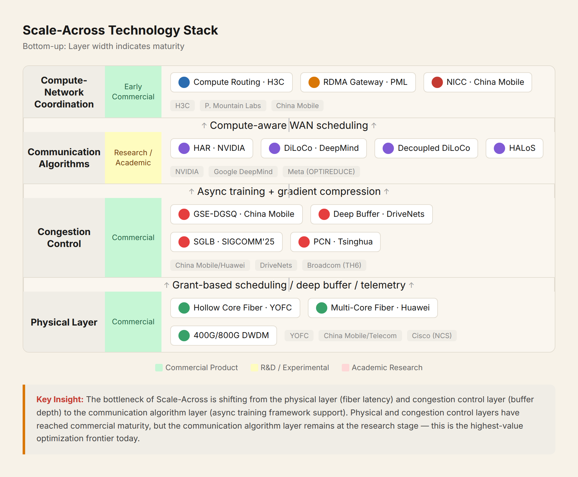
If §2 answers "why it must be done" and §3 answers "what the technical challenges are," §4 answers "what technical approaches are solving these challenges." The following sections unfold across four layers: physical layer, congestion control layer, communication algorithm layer, and compute-network co-design layer.
4.1 Physical Layer: Fiber Technology Is Pushing Boundaries
Hollow-Core Fiber: 30% Lower Latency, 90% Lower Loss
Solid-core fiber has a physical limit: light can only travel at 2/3 of vacuum speed, with signal attenuation of ~0.2 dB/km. Hollow-core fiber uses air as the transmission medium, solving both problems simultaneously: light speed approaches vacuum (30% lower latency), and loss drops to 0.05-0.1 dB/km (1/10th of traditional fiber).
China Mobile is at the forefront. In June 2024, it completed the first 800G hollow-core fiber transmission test network (between Shenzhen and Dongguan). The first commercial line was deployed in 2025, with Yangtze Optical Fibre (YOFC) as the sole winning bidder at a bid price of ~36,000 RMB per fiber-km (YOFC 2025 Semi-Annual Report / CFCF 2025 Summit disclosure). China Telecom followed closely, conducting two hollow-core fiber tenders in 2025 with price limits of 37,000-50,000 RMB per fiber-km.
The value of hollow-core fiber for Scale-Across is not cost savings—it is that the latency advantage over solid-core fiber scales with distance. 83 km saves ~0.26 ms (round trip, n=1.47 vs n=1.0); 300 km saves ~0.94 ms. Within a 1 ms budget, this is the difference between "cannot do sync" and "can try sync."
However, hollow-core fiber is still in its early commercial stage. Three engineering challenges limit its rollout speed:
- Mode coupling loss: Light propagates at the air-cladding interface in hollow-core fiber, making it extremely sensitive to bend radius. Traditional solid-core fiber can handle bend radii as small as 10 mm; hollow-core fiber must maintain a radius of 10-30 cm or more—otherwise mode coupling causes signal attenuation to spike. This imposes stringent requirements on existing conduit layouts.
- Splicing and connector technology: Splicing hollow-core fiber to traditional solid-core fiber produces 0.3-0.5 dB of splice loss (traditional fiber splicing is ~0.05 dB), which becomes non-negligible after accumulating splices over long-distance links.
- Mass production yield: The internal microstructure of hollow-core fiber (reflective ring structure) requires nanometer-level precision control. Currently, only a few manufacturers have mastered continuous production processes exceeding 10 km in length.
YOFC is one of the few known volume suppliers globally (CFCF 2025 Optical Connectivity Conference disclosure). These engineering challenges mean hollow-core fiber deployment will start with short-distance, high-value scenarios (such as same-city Scale-Across interconnection), then gradually expand to long-haul trunk lines.
Multi-Core Fiber: Parallelism Within a Single Fiber
Not speed improvement, but capacity expansion. 4-12 cores integrated into a single fiber, multiplying equivalent bandwidth several times. In March 2026, China Telecom collaborated with Huawei to complete the world's first multi-core-fiber-based distributed training field trial across multiple AI compute centers on the Guangzhou-Shenzhen route, at an interconnect distance of 409.61 km, achieving equivalent compute efficiency of over 97% versus centralized training. ITU-T SG15 is advancing MCF standardization; G.65x-series-compatible multi-core fiber standards are expected by 2028.
4.2 Congestion Control Layer: The Core Technical Barrier
The mainstream congestion control solution for AI training networks is ECN (Explicit Congestion Notification) plus PFC (Priority Flow Control), but these have fundamental flaws in cross-data-center scenarios. ECN is post-hoc intervention: marking packets after congestion occurs and signaling rate reduction—under 0.9 ms RTT, the response is severely delayed. PFC is hop-by-hop backpressure that can create a domino effect over long-distance links—congestion on one port can backpressure the entire network.
Meta reduced its reliance on DCQCN (an ECN-based congestion control protocol) in its 400G RoCE deployment, switching instead to PFC deep buffering plus congestion management at the collective communications library level (Meta Engineering Blog, "RoCE networks for distributed AI training at scale," 2024.8.5). This is an industry inflection signal: when ECN fails in long-distance large-scale scenarios, the entire congestion control paradigm needs rework.
| Solution | Core Idea | Key Difference from ECN/PFC | Source |
|---|---|---|---|
| GSE-DGSQ | Change from "push" to "pull" flow: source requests authorization before sending | Prevents congestion at the source rather than slowing down after congestion | China Mobile GSE (2023-2026) |
| INT-assisted congestion control | Embed telemetry metadata in packets for precise per-hop queue awareness | Proactive understanding of global network state | HPCC (Alibaba Cloud / SIGCOMM 2019), ICC (Tsinghua / 2025) |
| SGLB | SyncMesh protocol lets all switches share congestion information | Distributed global awareness, beyond just ECMP hashing | SIGCOMM 2025 |
| PCN | Receiver-driven congestion notification, rate reduction within one RTT | Sender does not wait for congestion marks, faster than ECN | Tsinghua / NSDI 2020 |
GSE-DGSQ "Pull" Mode
In 2023, China Mobile, together with industry partners, released the GSE (Global Scheduling Ethernet) technical architecture. Its core mechanism is DGSQ (Dynamic Global Scheduling Queue). Traditional Ethernet operates in "push" mode: the source starts sending and downstream switches passively receive. GSE switches to "pull" mode: the source first requests DGSQ authorization from the target egress, and only sends packet containers (PKTC) after receiving approval. Incast congestion is fundamentally avoided because the target port, at authorization time, already knows that the total incoming volume will not exceed its receiving capacity. PFC backpressure also becomes unnecessary—especially useful in cross-distance scenarios (long RTT no longer requires loop-based congestion control, since authorization completes before sending).
GSE has formed an open standards organization. Multi-vendor equipment interoperability testing was completed in 2024. At MWC March 2026, China Mobile released GSE-DCI (cross-data-center extension) along with the world's first 100T+ AI compute interconnection router prototype (115.2 Tbps). The equipment ecosystem includes Huawei, ZTE, Ruijie, and others.
The key advantage of GSE-DGSQ in cross-domain scenarios is that the authorization mechanism absorbs RTT asymmetry. In traditional "push" mode, if the target port is congested, the source can only sense this indirectly through PFC (one RTT later). On an 83 km link with 0.9 ms RTT, this means each AllReduce round could have hundreds of microseconds of congestion blind spot. GSE's "pull" mode eliminates this blind spot: authorization completes before data transmission begins, so the source knows the target port's reception capacity at the time it obtains authorization. The tradeoff is that authorization itself requires one control-plane RTT, but this RTT can overlap with the previous data transmission and does not increase critical-path latency.
4.3 Communication Algorithm Layer: Reducing Cross-Site Synchronization Volume
The core idea is not to make the network faster, but to let training continue even when the network cannot keep up.
Hierarchical AllReduce (NVIDIA NeMo Framework, 2025.5)
NVIDIA NeMo Framework 25.02 introduced Hierarchical AllReduce (HAR): first aggregate gradients within one data center, then synchronize the aggregated result across DCs. Cross-DC communication volume drops from O(N) to O(1). The concurrently released distributed optimizer architecture (Megatron-Core 0.11) reduces cross-DC synchronization frequency from every step to every N steps, while maintaining convergence quality.
OPTIREDUCE (NVIDIA + VMware, arXiv 2025)
An underappreciated contribution. OPTIREDUCE discovered that distributed deep learning has inherent fault tolerance to gradient loss: under common loss functions and optimizer configurations, losing a portion of gradients has an acceptable impact on convergence quality. This opens up a critical space for WAN link jitter scenarios: the option to "skip this synchronization" instead of waiting for retransmission.
Convergence Guarantees for Async Training
| Solution | Core Innovation | Convergence Guarantee | Communication Reduction | Source |
|---|---|---|---|---|
| DiLoCo | 500 steps (original default hyperparameter) of local SGDP then global sync | Empirically validated | ~500x | DeepMind 2023 |
| Decoupled DiLoCo | Decoupled "compute islands," async data flow | Empirically validated | Extremely low | DeepMind 2026.4 |
| HALoS | Hierarchical async local SGD + momentum | Convergence proven | Extremely low | arXiv 2025 |
| Streaming DiLoCo | Gradient compression from 16-bit to 4-bit | Empirically validated | 4x bandwidth savings | DeepMind 2026 |
(Note: "Empirically validated" means convergence was observed experimentally, but no formal proof exists yet.)
Decoupled DiLoCo, released April 23, is the most breakthrough advancement in async training. It does not make cross-DC synchronization faster—it fundamentally decouples computation. Training proceeds asynchronously on independent "compute islands," with information exchanged between islands through non-real-time data flows. A hardware failure on one island does not affect other islands' continued training; Gemma 4 validation shows convergence quality comparable to synchronous training. HALoS (arXiv 2025) further provides the first convergence proof for hierarchical async distributed optimization (including momentum), achieving 7.5x faster training convergence than DiLoCo in cross-regional environments.
A gap remains between academia and industry. Academia has been validating the feasibility of large-scale async training, while industry commercial products (DriveNets' deep buffer solution, Meta Prometheus) currently only support synchronous training. The reason is that the training framework layer (Megatron / DeepSpeed / JAX) does not yet offer mature async support for WAN scenarios—particularly the handling of loss terms that require global synchronization (such as moe_loss and z-loss) under async mode, which is still under investigation.
Quantifying the async training tradeoff clarifies the picture. The per-step communication overhead for sync DP is approximately 2 × model_size × bytes_per_param / bandwidth (RingAllReduce two-phase). For a 70B parameter model (fp16, 2 bytes/param) with 400 Gbps network bandwidth, per-step communication overhead is about 2 × 70 × 10⁹ × 2 × 8 / 400 × 10⁹ ≈ 5.6 s. If cross-DC bandwidth drops to 100 Gbps (typical long-haul DWDM single wave), per-step communication for sync DP rises to ~22.4 s—if the step computation time itself is only 2-3 s, the communication ratio degrades from ~65% to 88%+, which is effectively infeasible. With DiLoCo synchronizing once every 500 steps, the effective communication ratio drops to ~0.45%, but at the cost of 500 steps of parameter staleness. Decoupled DiLoCo further eliminates synchronous waiting time, but requires each compute island to independently maintain a full optimizer state (Adam momentum + variance, ~2× model size), nearly doubling memory overhead.
This is the core tradeoff across Scale-Across technology stack layers: physical layer acceleration (hollow-core fiber) and congestion control optimization (GSE) compress latency; the communication algorithm layer (async training) reduces synchronization frequency. Both must be applied together to achieve acceptable training efficiency in cross-domain scenarios.
4.4 Compute-Network Co-design Layer: Focus Area for Chinese Vendors
A distinctive feature of Chinese solutions is that network equipment vendors are not merely providing connectivity—they are attempting compute scheduling at the router level.
H3C's CR19000-X deterministic compute core router introduces the concept of "compute routing": the network layer not only forwards data packets but also senses compute load across sites, routing training tasks to the optimal compute node. This breaks the traditional role of "network as just a transport pipe." Purple Mountain Laboratories (in its August 2025 White Paper on "AI Large Model Cross-Domain Training Pooled Scheduling Technical Architecture") proposes a more systematic architecture: RDMA gateways deployed at WAN ingress wrap cross-domain training into local RDMA calls, with the endpoint side unaware of cross-DC existence. The upper layer coordinates three tiers: compute scheduling platform, storage scheduling, and network management. China Mobile's NICC (New Intelligent Computing Center) technical framework (2024-2026) defines five core technology directions: storage, compute, network, management, and efficiency.
4.5 Cloud Provider Approaches
North American cloud providers' investment in cross-domain training is primarily focused on internal infrastructure, with fewer technical details disclosed publicly than Chinese operators. AWS EFA (Elastic Fabric Adapter) supports cross-AZ RDMA communication, but AZ distances typically do not exceed 100 km, with the design goal being fault isolation rather than scale expansion. Azure's NCC (NVIDIA Collective Communications Library) integration in ND-series VMs remains experimental for cross-region training. GCP's GDCN (Google Distributed Cloud Networking) with Multislice Training is the most mature among the three.
SemiAnalysis noted in late 2025 that OpenAI is also pushing cross-domain training, but with a different strategy: OpenAI prefers to concentrate GPUs in as few campuses as possible (modular data centers + fast construction) rather than distributing and connecting them. This yields two technology paths: the "centralization school" (OpenAI, some hyperscalers) and the "distribution school" (Google, Chinese operators, with Meta gradually catching up).
§5 Global Scale-Across Deployment Roadmap
Before unfolding the table, let us first explain what the "97% equivalent compute" number actually means in practice. If a centralized cluster takes 30 days to train a model, 97% equivalent compute means cross-domain training takes 30 / 0.97 ≈ 30.9 days—an additional ~22 hours. For a trillion-parameter model with a typical training cycle of 3-6 months, this overhead is nearly negligible. But "97%" refers to throughput efficiency, not convergence efficiency—if async training leads to final model quality degradation (e.g., 0.02 higher final loss), that loss cannot be compensated by time. Therefore, Chinese operators all report that convergence quality is "consistent" with centralized training (final loss difference <0.5%) in their validations—this is the complete picture that gives these numbers meaning.
Notes on the "Efficiency" column: Different sources use different calculation methods. China Unicom/China Mobile use "equivalent compute" (training throughput comparison), China Telecom uses "training efficiency ratio." DriveNets' validation did not publish specific training efficiency. Meta Prometheus data is from SemiAnalysis analytical estimates. Under a unified methodology, operator validation results report a range of 95-98% equivalent single-cluster efficiency, indicating that cross-domain training compute loss at the 200 km level is not as high as originally anticipated.
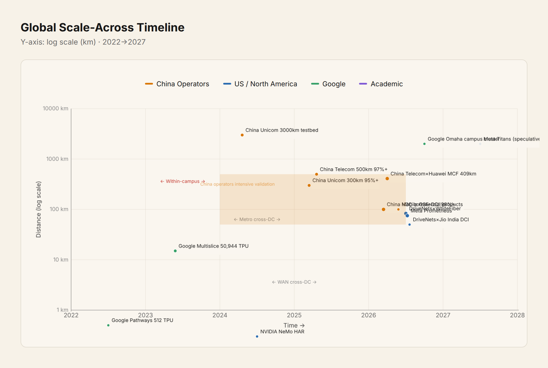
| Time | Player | Distance | Efficiency | Bandwidth | Technology Path | Notes |
|---|---|---|---|---|---|---|
| 2023 | Google Multislice Training | Cross-island (~15 km) | 97.2% throughput | - | Pathways async data flow | 50,944 TPU v5e training 32B params |
| 2024 | China Unicom | 3000 km | Test bandwidth utilization 20%→90% | - | Long-haul RDMA + lossless flow control | Shanghai→Ningxia testbed, fiber with repeaters |
| 2024 | NVIDIA NeMo | - | HAR communication savings ~50% | - | Hierarchical AllReduce | Software framework layer |
| 2025 | China Unicom | 300 km | 95%+ equivalent compute | 16:1 oversubscription ratio | OTN + precision flow control | Shanghai Lingang |
| 2025 | China Telecom | 500 km | 97%+ | - | Optical-electronic synergy | Wuqing, billion-parameter scale |
| 2026.3 | China Mobile | 100 km+ | 98%+ | 115.2T router | GSE-DCI proprietary protocol | MWC release |
| 2026.3 | China Telecom × Huawei | 409.61 km | 97%+ | MCF | Multi-core fiber field trial | Guangzhou→Shenzhen |
| 2026.5 | H3C | 100 km DCI / thousand-km cross-domain | 96% bandwidth utilization | 800G × 64 ports | S12500R-64EP + CR19000-X | Commercial product |
| 2026.7 | DriveNets × WhiteFiber | 83 km | Near single-node | 111.2 Tbps | Deep buffer + FSE + TH6 | First commercial deployment |
| 2026 | Meta Prometheus | 75-80 km campuses | - | 22 Pbps (campus total aggregate) | AIBB L3/L4 Superspine | SemiAnalysis estimate |
| 2026.7 | DriveNets × Jio | Same-city | - | 64×800G | Cisco NCS 1020J | India 800G DCI |
| ~2027 | Meta Titans | 2000 km | - | - | Async RL training | SemiAnalysis speculation, not officially confirmed |
Supplement: Google's Cross-Domain Training Roadmap
Google is the earliest company to systematically explore cross-data-center training in the industry. The 2022 Pathways paper (arxiv 2203.12533) first proposed an async distributed dataflow architecture, allowing training tasks to be split across TPUs in different islands, achieving 97.2% of synchronous training equivalent throughput in a 512-chip P2P DCN environment. In 2023, Multislice Training went live, demonstrating 50,944 TPU v5e chips connected into a single virtual cluster training a 32B parameter model—the largest publicly disclosed distributed training run in the world (Google Cloud Blog).
More importantly, there is Google's physical layout. Three campuses in Omaha-Council Bluffs-Papillion (Iowa) are spaced at approximately 10-15 miles apart, plus the Lincoln campus (Nebraska) at roughly 50 miles. These four campuses form a GW-scale training cluster in 2026. Three more campuses in Columbus (Ohio) also reached 1 GW scale by end of 2025. Google's MegaScaler is the earliest known sharder to have actually conducted synchronous training across campuses in production (based on Pathways).
Reading this table together with the global players reveals three clear trends:
Trend One: Cross-domain training within 200 km has approached engineering maturity. From China Unicom's 300 km at 95%+ in 2024 to DriveNets' 83 km near single-node performance in 2026, there are no fundamental technical barriers within 200 km. What remains to be solved are engineering deployment issues (fiber resources, equipment integration, adaptation with existing training frameworks) rather than network principles.
Trend Two: Technology routes are shifting from "pure network optimization" to "network + algorithm co-optimization." Attempts in 2024 focused on long-haul RDMA and lossless flow control (pure network layer). 2025-2026 began extending upward—NVIDIA NeMo with hierarchical AllReduce (communication algorithm layer), GSE-DCI with authorization-based scheduling (adding a new protocol layer), Decoupled DiLoCo with compute island decoupling (compute-network co-design). Multi-layer coordination from the physical layer to training strategy is the inevitable path.
Trend Three: Chinese operators' dense validation efforts are forming a de facto standard set. China Unicom, China Telecom, and China Mobile together completed at least 6 field trials across different distances and technology routes between 2024 and 2026, spanning from 100 km to 3000 km, and from OTN to hollow-core fiber to multi-core fiber. No other country has this density. Although each operator's technical parameters are coupled and testing methodologies are not yet directly comparable, this accumulated engineering experience itself constitutes a network effect.
§6 Assessment
6.1 Scale-Across Is Becoming the Third Formal Dimension of AI Networking
This is not a "special scenario" workaround. The triple pressures of power bottlenecks, equipment supply chains, and training scale are transforming Scale-Across from an optional approach into a standard component of AI infrastructure. A 650 Group analyst noted in a research report (July 2026 Ethernet AI Networking Market Update) that this is a new market that did not exist two years ago and has now formed over $100 billion in total addressable market. (Note: This figure represents Scale-Across's total related market TAM, including fiber, optical modules, installation and maintenance, not limited to switch hardware.)
6.2 Among Operators, China Leads in Validation and Deployment
Not because of superior technology, but because of different structural conditions. China's three major operators are 1-2 years ahead of North American cloud operator DriveNets (2026.7) and Meta (2026) in commercial-scale cross-domain training validation and deployment (2024-2026). (Note: Google is an exception—its 2022 Pathways paper already demonstrated cross-island training, and Multislice entered production in 2023.) Chinese operators are also more mature in distance (409 km vs 83 km) and efficiency (95-98% vs "near single-node"). Factors include the natural demand created by the Eastern Data Western Computing initiative, operator ownership of fiber networks, and clear policy-driven support.
Looking at the originality and ecosystem maturity of technology routes, the US has NVIDIA Spectrum-XGS's mature commercial ecosystem, while China has GSE's open standards organization. The technology gap between the two sides is not in 100 km-level deployment capability, but in standardization, ecosystem building, and productization maturity.
6.3 The Most Valuable Optimization Direction Is Not Traffic Engineering—It Is Async Support in the Training Framework Layer
From the analysis in §4, Scale-Across's bottleneck is shifting from "the network is not fast enough" to "the training framework does not support cross-WAN async mode." DriveNets' 0.9 ms is already very close to the 0.81 ms physical limit. Meta Prometheus's synchronous training within campuses is also nearly maximized. The more important step is to reduce latency sensitivity through better async training algorithms. Decoupled DiLoCo (2026.4) and HALoS's convergence proof point the direction; the next milestone should be the productization of these approaches into mainstream training frameworks (Megatron / DeepSpeed / JAX).
6.4 Looking Ahead
Three years from now, looking back, our current understanding of AI training clusters' "geographic constraints"—where the power is, how the fiber goes, when the transformer arrives—may be as basic to AI infrastructure engineers as today's understanding of GPU memory hierarchies (HBM2 → HBM3E → HBM4).
This constraint determines not only where training happens, but also feeds back into model architecture choices. When Scale-Across becomes a compulsory subject, AI infrastructure design will no longer be a one-way flow of "first choose the model, then build the network." It becomes a joint optimization across all three dimensions.
6.5 Competitive Landscape Implications
Scale-Across is rewriting the competitive rules of the AI infrastructure market. The competitive dimension for switches shifts from port density and backplane bandwidth to buffer depth, cross-domain scheduling capability, and fiber resources—DriveNets breaks ground with deep buffers, Chinese vendors differentiate with compute routing and GSE architecture. The accumulated advantages of traditional data center switch giants (Cisco/Arista/Juniper) in port density will not automatically extend to the Scale-Across domain.
A deeper implication: for GPU buyers, where the GPUs are matters more than how many GPUs you have. Two 50 MW clusters connected by 100 Tbps over 80 km may differ from a single-site 100 MW cluster by only 3-5% in training efficiency, but the time difference in obtaining power is years. This means the starting point for future AI infrastructure planning is no longer "how many cards to buy," but "where is the power, and can the fiber reach it."
Returning to the three dimensions at the beginning: Scale-Up solves "how fast the chip can compute," Scale-Out solves "how large the cluster can grow," and Scale-Across solves "where training can happen." The first two are technology problems; the third is a geography problem. The moment GPU cluster scale exceeded the power supply limit of a single site, AI infrastructure became not just an engineering problem, but a geographic-economic one.
Data Sources
- Gartner 2026 Data Center Infrastructure Forecast (published 2026.7.9)
- Wood Mackenzie, "US Power Transformer Lead Times, 2026 Update" (non-public report; 160-week transformer data cited from SemiAnalysis and Gartner analysis)
- SemiAnalysis, "The Future of Meta Superintelligence" (2026.7.9)
- DriveNets Blog, "Inside WhiteFlyer's Long-Distance Scale-Across Deployment" (2026.7.9)
- Meta Engineering Blog, "RoCE networks for distributed AI training at scale" (2024.8.5)
- NVIDIA Developer Blog, "Turbocharge LLM Training Across Long-Haul Data Center Networks with NeMo Framework" (2025.5.8)
- NVIDIA NIDA-006-2025 Standard Document (data on impact of packet loss rate on AI training network efficiency)
- Google DeepMind, "Decoupled DiLoCo: A new frontier for resilient, distributed AI training" (2026.4.23)
- arXiv 2506.04531, "HALoS: Hierarchical Asynchronous Local SGD over Slow Networks for Geo-Distributed LLM Training" (2025)
- arXiv 2604.21428, "Decoupled DiLoCo for Resilient Distributed Pre-training" (2026.4)
- arXiv 2203.12533, "Pathways: Asynchronous Distributed Dataflow for ML" (2022)
- arXiv 2310.06993, "OPTIREDUCE: Resilient and Tail-Optimal AllReduce for Distributed Deep Learning in the Cloud" (2025 update)
- OPTICA / Acta Optica Sinica, "Architecture, Key Technologies and Applications of Optical Interconnection for AI Computing" (2025.7)
- ACG Research, "TCO Comparison: Dark Fiber vs Leased Circuits at 100G and Beyond" (2025)
- Yangtze Optical Fibre (YOFC) 2025 Semi-Annual Report / CFCF 2025 Optical Connectivity Conference (China Telecom Research Institute disclosure)
- China Mobile GSE-DCI MWC 2026 Release (IT Home / Sina Tech, 2026.3.3)
- ZTE Technologies, "Scale-Up/Out/Across Three-Domain Synergy, Breaking Through Compute Limits" (2026.4)
- H3C NAVIGATE 2026 Press Release / AI Computing Network New Product Launch (2026.5.13)
- Purple Mountain Laboratories, "AI Large Model Cross-Domain Training Pooled Scheduling Technical Architecture White Paper" (2025.8)
- Cisco Blogs, "The Tipping Point: Managing the Cost of DCI in the AI Era" (2026.1)
- 650 Group, "Ethernet AI Networking Market Update, Q2 2026" (published July 2026, cited in DriveNets press release and Light Reading coverage)
This report does not constitute investment advice. Data as of July 16, 2026.