The Three Blind Spots of AI Observability
When your monitoring says "all green" while your AI systems quietly burn money, drift off track, and spiral out of control
Traditional APM tells you "200 OK, latency 250ms." What it doesn't tell you: this request cost $1.74 in tokens, the inference engine's KV Cache hit rate is under 20%, and the Agent went off track halfway through — everything after that was wasted. The harsher reality: research from UC Berkeley and others found that multi-agent systems fail 86.7% of the time in AppWorld tests [1] — and traditional monitoring has no idea.
A Paradox
In 2026, enterprise AI spending surpassed a trillion dollars, with network infrastructure taking an ever-growing share. Yet industry surveys reveal that most AI performance bottlenecks ultimately trace back to the network layer, not compute — and traditional monitoring tools are blind to this.
Salesforce's engineering team hit the same wall. Their Agentforce platform runs 60+ AI features for 600 users across 400+ million records. When an Agent misbehaved, engineers needed two weeks to pinpoint the problem. Not because the problem was complex — but because they couldn't see what was happening inside the Agent. They eventually built a dedicated Query-Driven Observability platform, cutting debugging time from two weeks to a single day.
This isn't a Salesforce-specific issue. It's a foundational infrastructure gap across the entire AI industry.
The "200 OK Syndrome" of Traditional APM
Traditional Application Performance Monitoring (APM) — Datadog, New Relic, Grafana — was designed for the request-response model:
Request arrives → Service processes → Response sent
Monitor: latency, error rate, throughput, CPU/memory utilization
This model worked perfectly in the web service era. But AI systems don't fit it at all.
A single AI request is not one operation — it's a decision chain. An Agent receives "analyze our competitors' pricing strategies." It needs to: search for competitor info → read pricing pages → extract data → analyze patterns → generate a report. Every step can fail, drift, or hallucinate. Traditional APM sees "200 OK, total time 45 seconds" — all fine.
But is it?
- Of those 45 seconds, the Agent spent 8 seconds on actual reasoning and 37 seconds waiting for API responses and retrying failed searches.
- It consumed 100,000 input tokens and 3,200 output tokens. At Claude Opus pricing ($15/$75 per M tokens), that's $1.74.
- About 80,000 of those input tokens were system prompt and tool definitions — the actual user prompt was only 800 tokens.
- The inference engine's KV Cache hit rate was under 20%, meaning most of the compute was recalculating things it had already calculated.
- At step 4, the Agent searched for the wrong competitor name. The remaining 6 steps all analyzed the wrong target.
Traditional APM can't see any of this. This isn't a tool deficiency — it's a generational gap in the observation model.
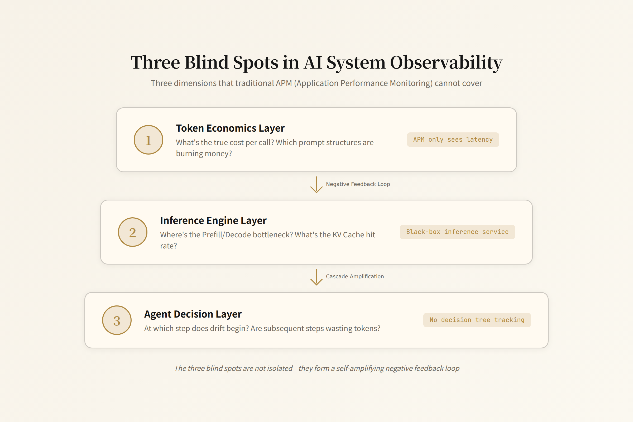
Three Blind Spots
The observability gap in AI systems breaks down into three layers. Each corresponds to a dimension that traditional monitoring completely misses:
Blind Spot 1: Token Economics — You Don't Know What You're Paying For
Most enterprises using AI APIs only look at their monthly bill total. But the breakdown behind that total is a black box:
- Prompt cost inflation: FutureAGI's analysis showed that in a typical Coding Agent workload (12 engineers / 8 MCP servers / 22 sessions/day), MCP protocol overhead (tool definitions + response serialization) accounts for 41–58% of total token spend [2]. Only 15–20% comes from actual user prompts. But you pay for 100% of the tokens.
- Marginal cost of context windows: Going from 4K to 32K context is relatively modest in cost, but from 128K to 1M is exponential. Chroma's Context Rot research found that accuracy begins degrading beyond 32K tokens. And Attention's O(n²) complexity means doubling context quadruples computation — measured long-context throughput can plummet 50x.
- The MoE pricing paradox: DeepSeek V3 has 671B total parameters but only activates 37B per inference (5.5%). It prices by activated parameters (¥2/M input, roughly 1/12 of GPT-4o). This is systematically eroding the pricing power of frontier models.
- The hidden cost of model routing: RouteLLM (LMSYS, 2024) showed 85% cost savings on MT-Bench while retaining 95% performance — but only 45% savings on MMLU [8]. Routing returns are highly task-dependent.
The reality of the token economics blind spot: You pay for tokens, but you don't know the value of each one. In a typical Agent workload, roughly 85% of input tokens are "infrastructure cost" (prompt templates, tool definitions). Only 15% is "value creation cost" (actual user intent and model output). Without token-level cost tracking, enterprise AI spend optimization is guesswork.
Blind Spot 2: The Inference Engine Black Box — 200 OK But 3x Slower
When inference services slow down, traditional monitoring tells you "GPU utilization 95%." But what does 95% GPU utilization mean? Is it compute-intensive operations maxing out Tensor Cores, or memory-bound operations waiting on HBM bandwidth?
Performance bottlenecks inside the inference engine span multiple layers:
Prefill/decode asymmetry. A single inference request has two phases: prefill (process the input prompt — digest all input tokens at once) and decode (generate output tokens one at a time). Prefill is compute-bound — the GPU's Tensor Cores run at full speed. Decode is memory-bound — each token generation requires reading the entire model weights from HBM, but the computation is tiny. This means the same GPU's prefill throughput can be 10–50x higher than its decode throughput.
The KV Cache storage dilemma. Transformer architecture requires caching the Key/Value matrices of all previous tokens. A 128-layer, 128-head model at 128K context has a KV Cache of ~128GB — exceeding a single H100's 80GB VRAM. This is why Agent workloads (routinely 100K+ token contexts) become an inference engine's nightmare.
MoE expert routing communication overhead. MoE models activate only a small subset of "experts" per inference, but all experts' weights must be resident. In multi-GPU deployments where different GPUs hold different experts, each inference may need cross-GPU weight fetches. This All-to-All communication overhead can account for 30–40% of total inference time in extreme cases.
Speculative decoding accept rate volatility. Use a small model to draft a few tokens, then let the big model verify — correct guesses give 2–4x speedup, wrong ones mean rollback. But accept rates vary dramatically by task: code generation might hit 70–85%, while open-domain creative writing can be as low as 30–40%. Traditional monitoring only sees "average 2x speedup," not which request types are dragging down the average.
Root cause of the inference engine black box: Inference is not a single operation — it's a complex interplay of prefill, decode, KV Cache access, expert routing, and attention computation. Traditional APM stops at "request-level" granularity, but inference optimization gains live at the "kernel level" — execution time and resource utilization of every CUDA kernel on the GPU. The granularity gap between these two is roughly 1000x.
Blind Spot 3: Agent Decision Paths — Drifting at Step 7
This is the deepest and least mature layer.
An Agent doing a task is not a single API call — it's a decision chain containing multiple reasoning steps and tool calls. Each step's output becomes the next step's input. If any step goes wrong, the error propagates and amplifies downstream.
Agent failure modes are fundamentally different from traditional software:
Semantic drift, not error codes. Traditional software fails with a 500 error. An Agent fails by producing text that looks reasonable — it picked the wrong tool but the call succeeded; it misinterpreted the return value and generated a "confident but wrong" conclusion. No error code, no exception. Traditional APM sees 200 OK, but the direction was already off.
Loop deadlock. An Agent can get stuck in a "search → read → search the same thing → read again" loop. Every step executes successfully (200 OK), but the entire chain is spinning in place. This kind of problem doesn't exist in traditional systems — traditional services don't "decide" to re-call an API they've already called.
Context bloat. Every step adds tool results to the context. By step 15, the context might be 200K tokens — and reasoning quality degrades significantly as context grows (the "Lost in the Middle" phenomenon). Longer context doesn't just cost more; it actively reduces quality.
Multi-Agent handoff information loss. Agent A finishes its part and hands results to Agent B. But B's context doesn't include A's reasoning process — only A's final output. Alternative approaches A considered but discarded, A's data quality assessments, A's concerns about edge cases — all lost. B makes the next decision with a heavily compressed version of A's understanding.
Root cause of the Agent decision path blind spot: The observation need shifts from "request tracing" to "reasoning tracing" — not "which services did this request pass through," but "what is this Agent thinking, why did it make this choice, what alternatives did it consider and reject." Traditional APM's distributed traces cannot express this semantic-level decision path.
These Three Layers Are Not Independent — They Compound
The three blind spots coexist in real systems and amplify each other:
- An Agent suffering from context bloat (Layer 3) causes per-inference token consumption to double (Layer 1)
- The inference engine, running low on KV Cache capacity (Layer 2), starts evicting cache entries, degrading inference quality
- Degraded quality forces the Agent to take more steps to complete the task (Layer 3), further increasing token consumption (Layer 1)
This is a negative feedback loop. Traditional monitoring can't see this loop at all — it only sees "request succeeded, took a while, GPU utilization high."

Who's Doing What
LLM Application Observability (Layers 1–2): Langfuse (open source, ClickHouse backend) is the most mature option. Arize Phoenix has an edge among ML engineers. Both build on OpenInference's OpenTelemetry semantic conventions — the foundation for interoperability between different tools.
Inference Engine Profiling (Layer 2): Graphsignal does continuous high-resolution profiling, breaking inference into fine-grained timelines of prefill / decode / KV Cache / expert routing. vLLM and SGLang are also enhancing their built-in metrics. A more ambitious direction is autodebug — an autonomous agent that deploys inference services → collects telemetry → analyzes bottlenecks → auto-tunes configuration → redeploys, in an infinite loop.
Agent Observability (Layer 3): This is the least mature but most valuable direction. agent-run is trying to define an open standard for Agent observation. Atla does real-time visualization of Agent thoughts and tool calls. Deconvolute takes a security angle, building a policy-as-code firewall for MCP tool calls. But no tool in this space has reached "Langfuse-level" de facto standard yet.
Building End-to-End Observability: Global View, Phased Refinement
The three-layer blind spot analysis tells us what to observe. The real challenge is: how should an organization systematically build AI observability capabilities? Not piecemeal tool installation, but starting from a global architecture and refining in phases.
What to Observe at Each Layer
| Layer | Core Focus | Key Question | Typical Observables |
|---|---|---|---|
| Layer 1: Tokens & API | Cost and usage | "Where's the money going? Is it worth it?" | API calls, token composition, model routing, prompt caching |
| Layer 2: Inference Engine | Performance and efficiency | "What's the GPU doing? Why is it slow?" | Prefill/decode latency, KV Cache, attention kernel, MoE scheduling |
| Layer 3: Agent Decisions | Quality and correctness | "Did the Agent take the right path? Which step went wrong?" | Step traces, tool calls, drift detection, handoff quality |
Detailed observation matrices for each layer are in the respective Deep Dive articles. But the three layers are not independent multiple-choice options — they are projections of the same request at different granularities.
End-to-End: One Request Traversing All Three Layers
Imagine a user sending "analyze competitor pricing." From entry to completion, this request traverses all three layers:
User Request
  |
  |- Layer 1: API Gateway logs HTTP request
  |    -> token_count, model, cost, latency
  |    -> "This call cost $0.03, used GPT-4o"
  |
  |- Layer 1: Application middleware breaks down tokens
  |    -> system_prompt: 3000 / tools: 1500 / history: 8000 / user: 200
  |    -> "95% is infrastructure tokens"
  |
  |- Layer 2: Inference engine processes request
  |    -> prefill: 320ms (compute-bound) / decode: 3850ms (memory-bound)
  |    -> KV Cache hit rate: 60% / batch_size: 24
  |    -> "KV Cache is adequate, decode is the bottleneck"
  |
  |- Layer 3: Agent executes 15-step task
  |    -> Steps 1-3: correct exploration / Step 4: confuses competitor product lines
  |    -> Next 11 steps based on wrong premise / token waste rate: 81%
  |    -> "Agent went off track at Step 4"
  |
  `- Returns result (looks correct, actually wrong)
Key insight: Traditional monitoring only sees the final step — "request succeeded, took 45 seconds." Three-layer observability tells you: this request cost $1.74 (Layer 1), of which 81% of tokens were wasted on a wrong path (Layer 3), and the inference engine itself had no bottleneck (Layer 2).
Unified Trace ID: Connecting All Three Layers
Three-layer observability data is scattered across different tools — Langfuse records token costs, vLLM Prometheus records engine metrics, agent-run records step traces. Without correlation, you can only view three dashboards separately and manually piece together causality.
The solution is a unified Trace ID spanning all three layers:
HTTP Request (trace_id: abc123)
  |
  |- OTel Span: llm.call (trace_id: abc123, span_id: 001)
  |    attributes: model=gpt-4o, tokens=87000, cost=$1.74
  |
  |- OTel Span: inference.prefill (trace_id: abc123, span_id: 002, parent: 001)
  |    attributes: duration=320ms, input_tokens=35200
  |
  |- OTel Span: inference.decode (trace_id: abc123, span_id: 003, parent: 001)
  |    attributes: duration=3850ms, output_tokens=800, kv_cache_hit=60%
  |
  |- OTel Span: agent.step.4 (trace_id: abc123, span_id: 004, parent: 001)
  |    attributes: type=tool_call, tool=web_search, drift_score=0.3
  |
  `- OTel Span: agent.step.5-15 (trace_id: abc123, span_id: 005-015)
      attributes: wasted_tokens=161400, drift_detected=true
OpenTelemetry + OpenInference is driving this correlation standard. Once all three layers share a trace_id, you can:
- Billing anomaly → automatically locate which trace and which step burned the tokens
- Inference latency anomaly → automatically find whether the corresponding Agent step was spinning idle
- Agent drift → automatically check whether the inference engine had insufficient KV Cache at that moment
Build Cadence: Three Phases, Incremental
Don't try to build all observability capabilities at once. Follow this cadence:
Phase 1 (Weeks 1–2): Cost Visibility
- Deploy API client wrappers to log token composition and cost per call
- Integrate Langfuse (or Phoenix) for basic LLM call tracing
- Output: monthly bills broken down by application / department / user — know where the money goes
- Maps to foundational Layer 1 capabilities
Phase 2 (Weeks 3–6): Engine Transparency
- Enable vLLM Prometheus exporter to collect TTFT/TPOT/KV Cache metrics
- Deploy DCGM exporter to collect GPU utilization / power / bandwidth
- Build Grafana dashboards showing request-level and engine-level metrics side by side
- Output: able to answer "why was this request 3x slower"
- Maps to foundational Layer 2 capabilities
Phase 3 (Weeks 7–12): Decision Traceability
- Instrument OTel spans in the Agent runtime (one span per thought / tool call / error)
- Implement drift detection (start with behavioral pattern anomalies — low cost)
- Deploy Deconvolute or similar tools for tool-call auditing
- Output: able to answer "at which step did the Agent drift, and how many tokens were wasted"
- Maps to foundational Layer 3 capabilities
Continuous iteration:
- After completing all three phases, circle back to connect them via unified trace ID
- Add semantic drift detection (high cost, save for last)
- Explore automated tuning directions (AVO, adaptive batching)
Observability Is Not the Goal — Intervention Is
The endgame of an observability system is not three pretty dashboards, but a closed-loop control system:
Observe → Diagnose → Decide → Execute → Verify
- Observe: three-layer metrics + trace + log
- Diagnose: anomaly detection + root cause analysis (cross-layer correlation)
- Decide: automated or manual optimization strategy
- Execute: adjust routing, scale up/down, modify prompts, correct the Agent
- Verify: did the metrics improve?
The speed at which this loop runs determines the operational efficiency of an AI system. In traditional software, the loop cycle is measured in "days" (alert → investigate → fix → deploy). In AI systems, the goal is to compress it to "minutes" or even "seconds" — that's the ultimate value of the autodebug direction.
The Biggest Gap
Observability tools are emerging, but one structural gap remains unfilled: correlation across the three layers.
When an Agent task's monthly bill spikes (Layer 1 anomaly), you can't automatically trace it to a drop in the inference engine's KV Cache hit rate (Layer 2), which forced the Agent to take more steps to complete tasks (Layer 3). Observability data for each layer lives in separate tools, with no unified trace ID tying them together.
OpenTelemetry + OpenInference is attempting to build this correlation — from HTTP request to LLM call to inference engine metrics to Agent step — but current implementations are far from complete. This may be the biggest product opportunity in AI infrastructure for 2026–2027.
The Endgame: From "Seeing Problems" to "Fixing Them Automatically"
The ultimate goal of observability is not post-hoc analysis — it's real-time intervention.
When the system detects an Agent in a loop deadlock → automatically inject "You seem to be searching for the same information repeatedly. Try a different approach." When KV Cache hit rate drops below threshold → automatically adjust batching strategy or enable cross-node KV Cache sharing. When token cost spikes → automatically route to a cheaper model or compress the prompt.
This is the autodebug endgame — observability evolving from a separate observation layer into a self-optimizing feedback loop for the system itself. Inference engines shift from "configure then run" to "self-optimize during runtime." Agents shift from "manual debugging" to "automatic drift detection and correction."
Until that day arrives, the vast majority of AI systems are running without these three layers of observability — not because they lack monitoring, but because the monitoring dimensions don't match how AI actually works.
References
[1] Berger et al., "Why Do Multi-Agent LLM Systems Fail?" arXiv:2503.13657 (2025). UC Berkeley & Intesa Sanpaolo. Introduces MASFT (Multi-Agent System Failure Taxonomy), identifying 14 failure modes across 3 categories.
[2] FutureAGI, MCP Token Overhead Analysis. Representative workload: 12 engineers / 8 MCP servers / 22 sessions per day / 30 turns per session.
[3] Osmulski et al., "RouteLLM: Learning to Route LLMs with Preference Data", arXiv:2410.02062 (2024). LMSYS Org.
This article is the main entry of the AI Observability series. Three subsequent Deep Dives will explore Token Economics, Inference Engine Internals (down to the CUDA kernel level), and Agent Decision Path Observability.