Inside the Inference Engine
From Prefill to CUDA Kernel — a Millisecond-Level Breakdown of an Inference Request
Deep Dive 2 / 3 · This article is the second deep dive into The Three Blind Spots of AI Observability, focusing on the inference engine black box. We go down to the CUDA kernel level.
The Lifecycle of a Request
A user sends a message: "Summarize the core contributions of this paper."
The attached paper PDF is parsed into 32,000 tokens. Adding the system prompt and tool definitions, the total input is 35,200 tokens. The model needs to generate roughly 800 tokens of summary.
From the user hitting Enter to receiving the complete response, the total time is 4.2 seconds. What is the GPU actually doing during those 4.2 seconds?
| Phase | Duration | Share | Notes |
|---|---|---|---|
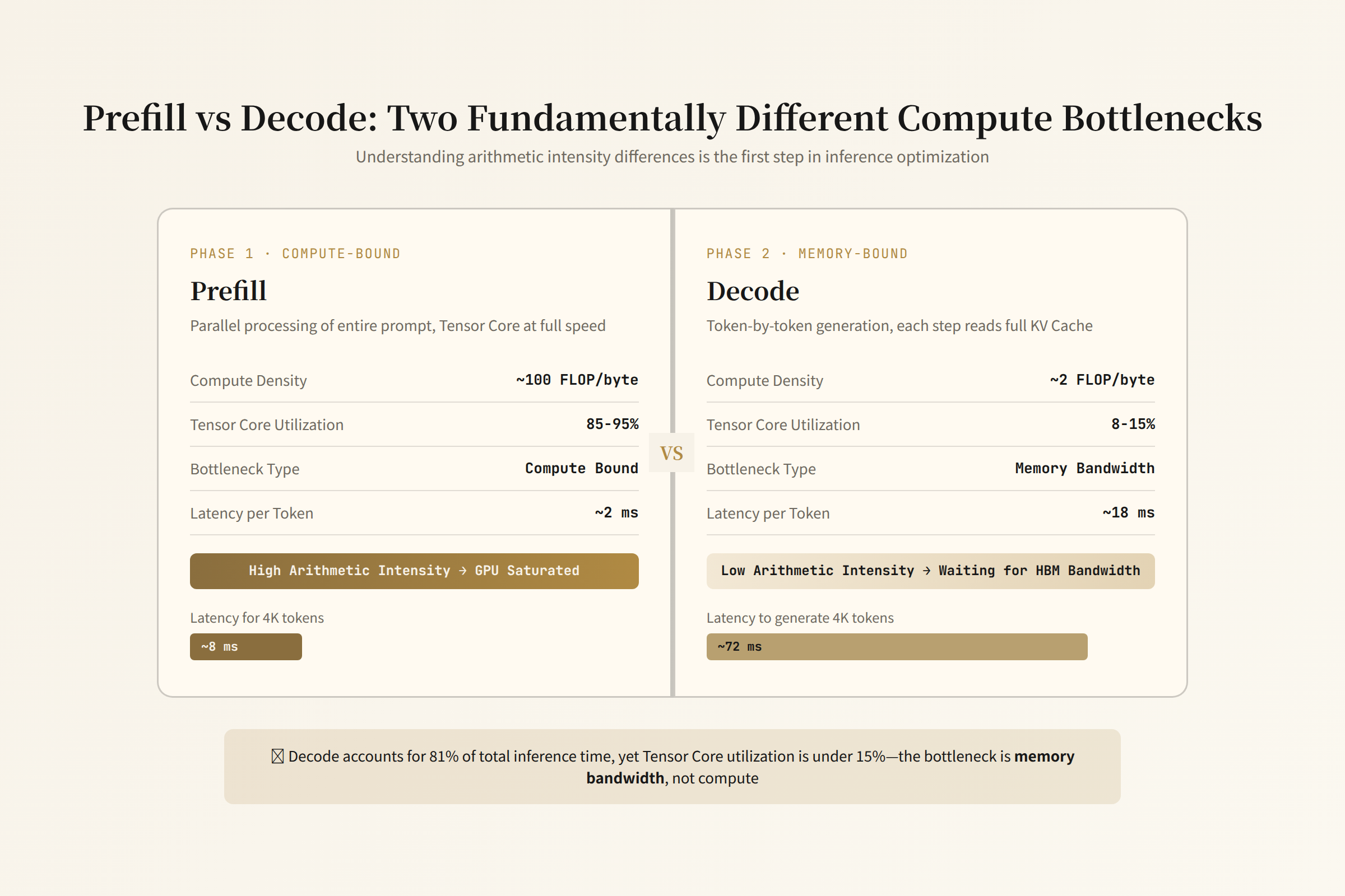
| Prefill | 320ms | 7.6% | 35,200 input tokens processed at once (compute-bound) |
| Decode | 3,850ms | 91.7% | 800 output tokens generated one by one, avg 4.8ms/token (memory-bound) |
| Network I/O | 30ms | 0.7% | HTTP/TCP round trip |
| Total | 4,200ms | 100% |
A seemingly simple request maps to hundreds of CUDA kernel calls on the GPU. Crack open the 4.2-second "black box" and you find four phases: Prefill, Decode, Attention, and MoE Expert Dispatch. Each phase has entirely different bottlenecks.
Prefill: A Compute-Bound Parallel Feast
35,200 Tokens Fed In All at Once
During the prefill phase, the model processes all 35,200 input tokens in a single pass. For each token, the model needs to:
- Embedding Lookup: Map token IDs to vectors
- N Transformer Blocks, each containing:
- Self-Attention computation
- MLP (Feed-Forward Network) computation
- LM Head: Final projection to vocabulary, computing the probability distribution for the next token
The defining characteristic of prefill is extremely high parallelism — all 35,200 tokens can be processed simultaneously. This means the GPU's Tensor Cores can be fed large matrix multiplications (GEMMs).
GEMM Kernel: Tensor Core's Home Turf
The core computation in Transformers is matrix multiplication. For an attention projection with hidden_dim=8192 and batch_size=35200 (token count):
Input matrix X:  [35200, 8192]   ← input embeddings
Weight matrix W: [8192, 8192]    ← model parameters
Output matrix Y:  [35200, 8192]   ← projected output

Y = X × W

FLOPs: 2 × 35200 × 8192 × 8192 ≈ 4.73 TFLOPS
A single matrix multiplication: 4.73 TFLOPS. A 128-layer model has 6 major linear projections per layer (Q/K/V/O + MLP up + MLP down). Total prefill computation: approximately 3.6 PFLOPS (note: MLP layer dimensions are typically 4x hidden_dim, so actual FLOPS are higher; this is a conservative estimate).
H100's FP16 Tensor Core peak throughput is 989 TFLOPS (dense), or 0.989 PFLOPS. In theory, 3.6 PFLOPS should take ~3.6ms. But actual prefill takes 320ms — about 90x slower. Why?
Because Attention computation isn't pure GEMM. There's Softmax, LayerNorm, residual connections — all memory-bound operations. Their computational density (FLOPs/Byte) falls well below the Tensor Core's efficiency knee, so the GPU spends most of its time waiting for data to move from HBM to SRAM.
From the CUDA Kernel Perspective
Kernel composition during prefill (using vLLM + Flash Attention as an example):
| Kernel | Purpose | Time Share | Bottleneck Type |
|---|---|---|---|
| GEMM (QKV Projection) | Project to Q/K/V matrices | 18% | Compute |
| Flash Attention Kernel | Self-Attention computation | 35% | Memory (SRAM/HBM) |
| GEMM (Output Projection) | Attention output projection | 8% | Compute |
| GEMM (MLP up-projection) | MLP first layer expansion | 15% | Compute |
| Element-wise (Activation) | SiLU/GELU activation functions | 5% | Memory |
| GEMM (MLP down-projection) | MLP second layer compression | 14% | Compute |
| LayerNorm + Residual | Normalization and residual connection | 5% | Memory |
Flash Attention is the single most expensive kernel (35%) — which seems counterintuitive, since Flash Attention's design goal is to reduce HBM access. The answer: while Flash Attention eliminates the O(n²) HBM read/writes of standard Attention, it remains the most memory-access-intensive operation in the pipeline. During prefill (long sequences), Attention's memory access volume still dominates.
The HBM Bandwidth Wall
The most critical concept for understanding inference engine bottlenecks is the memory wall — the bandwidth limitation of HBM (High Bandwidth Memory).
H100 key specs:
HBM bandwidth: 3.35 TB/s
FP16 Tensor Core: 989 TFLOPS (dense) / 1979 TFLOPS (sparse)

Arithmetic intensity knee ("roofline", FP16 dense):
  989 TFLOPS ÷ 3.35 TB/s = 295 FLOPS/Byte
This means: for every 1 byte read from HBM, you need to perform ≥295 floating-point operations to keep Tensor Cores saturated. If arithmetic intensity falls below 295 FLOPS/Byte, the GPU starves for memory — this is memory-bound.
The decode phase is the extreme case of exactly this scenario.
Decode: The Memory-Bound, Per-Token Marathon
The Life of a Token
During decode, the model generates output tokens one at a time. Each token requires a complete forward pass through the entire model — but batch_size is only 1 (or however many active requests are in the current batch).
For a single token's forward pass:
Input vector x:  [1, 8192]
Weight matrix W: [8192, 8192]
Output vector y:  [1, 8192]

y = x × W

FLOPs: 2 × 1 × 8192 × 8192 ≈ 134 MFLOPS
HBM read: 8192 × 8192 × 2 bytes (FP16) = 134 MB
Arithmetic intensity: 134 MFLOPS ÷ 134 MB = 1 FLOP/Byte
This is far below H100's knee of 295 FLOPS/Byte. Tensor Core utilization is ~0.34% of theoretical peak. 99.7% of the time is spent waiting for HBM to deliver the weights.
This is why the decode phase is called memory-bound — not because compute isn't fast enough, but because memory bandwidth can't feed the compute units.
Why Decode Is Slow But Not Power-Hungry
GPU power consumption during decode is actually lower than during prefill — because the Tensor Cores are mostly idle. HBM is reading model weights at high speed, but the compute units are waiting. It's like an F1 car stuck in city traffic — the engine is powerful but can't move.
This is also why continuous batching is critical for inference throughput: merging multiple decode requests into one large batch turns GEMV (matrix-vector multiplication) into GEMM (matrix-matrix multiplication), pulling arithmetic intensity from 1 FLOP/Byte to 10–50 FLOPS/Byte. The same weight matrix is read once, serving multiple requests — HBM bandwidth gets amortized.
Decode Kernel Composition
| Kernel | Purpose | Time Share | Difference from Prefill |
|---|---|---|---|
| GEMV (QKV Projection) | Single token Q/K/V projection | 12% | Prefill uses GEMM → here it's GEMV |
| Attention (with KV Cache) | Current token attending to historical KV | 20% | No Flash Attention needed, sequence length=1 |
| GEMV (Output Projection) | Attention output | 5% | |
| GEMV (MLP up/down) | MLP computation | 35% | For MoE models, this is expert dispatch |
| Memory Copy (KV Cache Write) | Writing current token's KV to cache | 8% | Doesn't exist in prefill |
| LayerNorm + Residual | Normalization | 10% | Memory-bound share is higher |
| AllReduce (TP) | Cross-GPU sync for Tensor Parallelism | 10% | Only with multi-GPU |
The Attention kernel during decode is completely different from prefill — prefill is O(n²) full attention, decode only needs to compute the current token's attention against all historical tokens (O(n)), since the attention between historical tokens was already computed during prefill.
Flash Attention: IO-Aware Attention
The Problem with Standard Attention
Standard Self-Attention computation:
S = Q × K^T     [n, n] — Attention Score matrix
P = softmax(S)   [n, n] — Attention Weight matrix
O = P × V        [n, d] — Output matrix
The problem: S and P are both [n, n] matrices. When n=35,200 (input token count), the S matrix size = 35200 × 35200 × 4 bytes (FP32) = 4.7 GB. This matrix needs to be written to HBM, read back for softmax, written to HBM again, and read back for P×V.
Standard Attention HBM access: O(n² + nd). For long sequences, n² dominates.
The Flash Attention Solution
Flash Attention (Dao et al., 2022, arXiv:2205.14135) core insight: don't write the [n,n] matrix to HBM. Split Q, K, V into blocks, load them into SRAM (on-chip cache), compute attention inside SRAM, and only write the final result to HBM.
SRAM size: ~228 KB/SM (H100)
HBM bandwidth: 3.35 TB/s

Flash Attention:
  Block size: block_size × block_size (typically 128×128)
  Load Q[i:i+B], K[j:j+B], V[j:j+B] into SRAM per block
  Compute S = Q×K^T, softmax(S), O += P×V inside SRAM
  Write only O to HBM

HBM access: O(n²d / M), where M is SRAM size
For n=35,200, d=128, M=64KB:
Standard Attention HBM read/write: O(n²) × 4 bytes = 35200² × 4 ≈ 4.96 GB
Flash Attention HBM read/write: O(n²d/M) ≈ 4.96 GB × 128 / 64KB ÷ 4 ≈ 2.4 MB
HBM access reduced ~500x. This is why Flash Attention dramatically speeds up long sequences — not by reducing computation, but by reducing memory access.
Flash Attention v2 Improvements
Flash Attention v2 (Dao, 2023, arXiv:2305.09426) optimizations:
- Reduced non-matmul FLOPs (rescale operations in softmax)
- Optimized parallelism — across the sequence dimension rather than the batch dimension
- Better warp-level workload distribution
On H100, Flash Attention v2 processing 8K sequences can reach ~190 TFLOPS (FP16 dense), about 19% of H100's FP16 dense peak (989 TFLOPS).
Flash Attention 3: Asynchronous Parallelism on Hopper
Flash Attention 3 (Tri Dao, 2024.07, arXiv:2407.08691) was redesigned from the ground up for the NVIDIA Hopper architecture (H100/H200) [1]. While FA2 runs on H100, it doesn't leverage Hopper's new hardware features. FA3's core breakthroughs are in three areas:
1. WGMMA Instructions + Asynchronous Execution Pipeline
Hopper introduces WGMMA (Warp Group Matrix Multiply-Accumulate) instructions — a single instruction that completes large matrix multiplication and accumulates directly into registers without first transiting through shared memory. FA3 executes both Q×K^T and P×V using WGMMA, and builds a three-stage asynchronous pipeline:
Stage 1: TMA asynchronously loads the next Q/K/V block from HBM to shared memory
Stage 2: WGMMA executes matrix multiplication for the current block (Q×K^T)
Stage 3: Softmax + accumulation (P×V) for the previous block

Three stages run in parallel on different warp groups
→ Computation and data movement fully overlap
Key insight: TMA (Tensor Memory Accelerator) is Hopper's hardware DMA engine that can complete HBM↔SRAM copies without occupying SM compute resources. In FA2, data movement and computation are serial; FA3 achieves true asynchrony through TMA.
2. Warp Specialization
FA3 splits GPU warps into two roles:
- Producer warps: Handle TMA async loads, moving data from HBM to SRAM
- Consumer warps: Handle WGMMA computation, performing matrix multiplication on SRAM data
The two groups synchronize asynchronously via barriers — producers signal consumers when enough data is ready, consumers signal producers when they're done and the buffer can be overwritten. This division of labor avoids the resource contention that occurs in FA2 when all warps do the same thing.
3. FP8 Low-Precision Support
FA3 supports FP8 input (e4m3 and e5m2), leveraging Hopper's FP8 Tensor Cores. In FP8 mode, throughput approaches 1.2 PFLOPS — the highest attention throughput achievable on a single H100.
Measured results: 740 TFLOPS in FP16 (75% of H100's FP16 dense peak of 989 TFLOPS), and close to 1.2 PFLOPS in FP8 [1]. By comparison, FA2 on H100 only reaches ~19% of peak — FA3 lifts utilization from 19% to 75%, effectively quadrupling theoretical throughput on the same card.
Flash Attention 4: Native Blackwell
Algorithm-Kernel Co-Design
Flash Attention 4 (Tri Dao's team, 2026.03, arXiv:2603.05451) is a product of the Blackwell architecture (B200/GB200) [3]. FA3 runs on Blackwell but doesn't exploit any of its new hardware features. FA4 is not a simple port — it's an algorithm-kernel co-design, meaning the attention algorithm itself is modified to fit hardware characteristics.
FA4's core insight: standard Flash Attention requires a global rescale of the output accumulator after processing each tile's softmax. This rescale reads and modifies the entire output accumulator — a memory-bound operation whose cost grows sharply with larger tile sizes. FA4 uses two algorithmic tricks to bypass it.
Trick 1: Conditional Softmax Rescaling
FA4 proves at the algorithm level that ~90% of inter-tile rescales are unnecessary — they're only needed when a tile's maximum logit significantly exceeds all previous tiles. FA4 adds a lightweight conditional check in the kernel, skipping rescales for tiles that don't need them. This is not an approximation — the result is mathematically identical to standard Flash Attention; it simply exploits the mathematical properties of softmax to avoid redundant computation.
Trick 2: Polynomial Approximation of Exponential
The exp() in softmax requires multiple instructions on a GPU. FA4 replaces it with a Chebyshev polynomial approximation, with negligible precision loss (< 0.1%) but significantly fewer instructions. This is another example of algorithm-kernel co-design: using polynomial approximation requires adjusting the algorithm's numerical stability strategy.
Blackwell Hardware Exploitation
FA4 deeply utilizes Blackwell's new hardware features:
- TMEM (Tensor Memory): A new memory hierarchy introduced in Blackwell — faster and larger than shared memory. FA4 places accumulators in TMEM, avoiding frequent writebacks to SRAM
- 2-CTA MMA Mode: Blackwell's Cooperative Thread Arrays can collaboratively execute matrix multiplication. FA4 uses larger tile sizes to fully exploit this mode
- Fully Asynchronous MMA: All matrix multiply operations are asynchronous, completely decoupling computation from data movement
Performance: Redefining the Attention Ceiling
B200 BF16 measured: 1613 TFLOPS (71% of B200 BF16 peak) [3]. What does this number mean?
For context:
- 1.1–1.3× faster than cuDNN 9.13's optimized attention kernel
- 2.1–2.7× faster than Triton-implemented Flash Attention
- More than double FA3's 740 TFLOPS on H100
CuTe-DSL: Python-Native Implementation
An engineering highlight of FA4: it's implemented in CuTe-DSL (Cutlass Tensor DSL) — a CUDA kernel DSL embedded in Python. Compilation is 20–30× faster than traditional C++ templates (CUTLASS), with equivalent performance. Kernel developers can iterate in Python without waiting 10 minutes for C++ compilation.
Worth noting: NVIDIA's AVO (Agentic Variation Operator) — an AI agent that automatically generates and optimizes GPU kernels — produced a variant that's 10.5% faster than FA4's hand-written kernel on attention [7]. This signals that kernel optimization is transitioning from human craft to AI search space.
KV Cache: HBM's Gravity
The Physical Size of KV Cache
For a model with 128 layers, 128 heads, head_dim=128, the KV Cache per token:
KV Cache/token = 2 (K+V) × 128 (layers) × 128 (heads) × 128 (head_dim) × 2 (FP16 bytes)
               = 2 × 128 × 128 × 128 × 2
               = 8 MB/token
Actual values vary by model. Using common large models as reference:
| Model | Layers | KV Cache/token (FP16) | 8K context | 128K context |
|---|---|---|---|---|
| Llama-3 70B | 80 | 320 KB | 2.5 GB | 40 GB |
| GLM-5.2 | 128 | ~1 MB | 8 GB | 128 GB |
| DeepSeek V4 (MoE) | ~96 | ~750 KB | 6 GB | 96 GB |
A single H100 has only 80GB HBM. 128K context KV Cache already exceeds single-card capacity.
PagedAttention: vLLM's Solution
vLLM's core innovation is PagedAttention — borrowing the virtual memory paging mechanism from operating systems to manage KV Cache.
Traditional approach:
  Pre-allocate contiguous HBM space for max_context_length per request
  → Internal fragmentation (allocated but unused) + external fragmentation (gaps between requests)

PagedAttention:
  Split KV Cache into fixed-size blocks (typically 16 tokens/block)
  Each request maps to physical blocks via a block table
  Allocate on demand — as many blocks as tokens generated
Result: KV Cache memory utilization jumps from ~40% (contiguous allocation + fragmentation) to ~95%. The same GPU can serve 2–4x more concurrent requests. SGLang's PD disaggregation architecture (Prefill-Decode Disaggregation) further separates prefill and decode onto different instances, transferring KV Cache via RDMA one-sided writes. AMD's official blog measured that PD disaggregation improves Goodput by up to 6.9x on Agent control and RAG tasks (95th percentile SLO), and 2.2x on decode-heavy scenarios [2].
From the CUDA kernel perspective, PagedAttention requires a custom attention kernel — because KV Cache is no longer contiguous memory, the kernel needs to look up physical addresses via the block table during every attention computation. vLLM uses xformers' memory-efficient attention as a base, with a paged version implemented on top.
MLA: Solving KV Cache at the Architecture Level
PagedAttention solves the KV Cache management problem but doesn't reduce its size. DeepSeek V3 took a different route: compressing KV Cache at the model architecture level — MLA (Multi-Head Latent Attention) [4].
MLA's core idea: in standard MHA, each head has independent K and V vectors, and KV Cache grows linearly with head count. MLA compresses K and V into a low-dimensional latent vector. During inference, only this compressed vector is cached; it's decompressed back into full K and V when needed.
Standard MHA KV Cache (per token):
  2 × n_layers × n_heads × head_dim × 2 bytes

MLA KV Cache (per token):
  n_layers × kv_latent_dim × 2 bytes
  (kv_latent_dim ≈ head_dim, far less than n_heads × head_dim)
The effect is dramatic: for DeepSeek V3, KV Cache shrinks from ~10 GB / 1000 tokens to ~0.67 GB / 1000 tokens — a 93% reduction [4]. The same GPU memory can now support 14× longer contexts or 14× more concurrent requests.
DeepSeek open-sourced FlashMLA — a decoding kernel specifically optimized for MLA (github.com/deepseek-ai/FlashMLA):
- 3000 GB/s memory bandwidth utilization on H800
- 580 TFLOPS BF16 compute throughput
- Paged KV Cache support (block size 64), consistent with PagedAttention principles
MLA's trade-offs include additional training complexity (learning compression/decompression matrices) and incompatibility with standard Flash Attention kernels (requiring dedicated kernels like FlashMLA). But a 93% KV Cache reduction far outweighs these costs. Expect most new models released in 2026–2027 to adopt MLA or similar architectures.
Multi-Level KV Cache
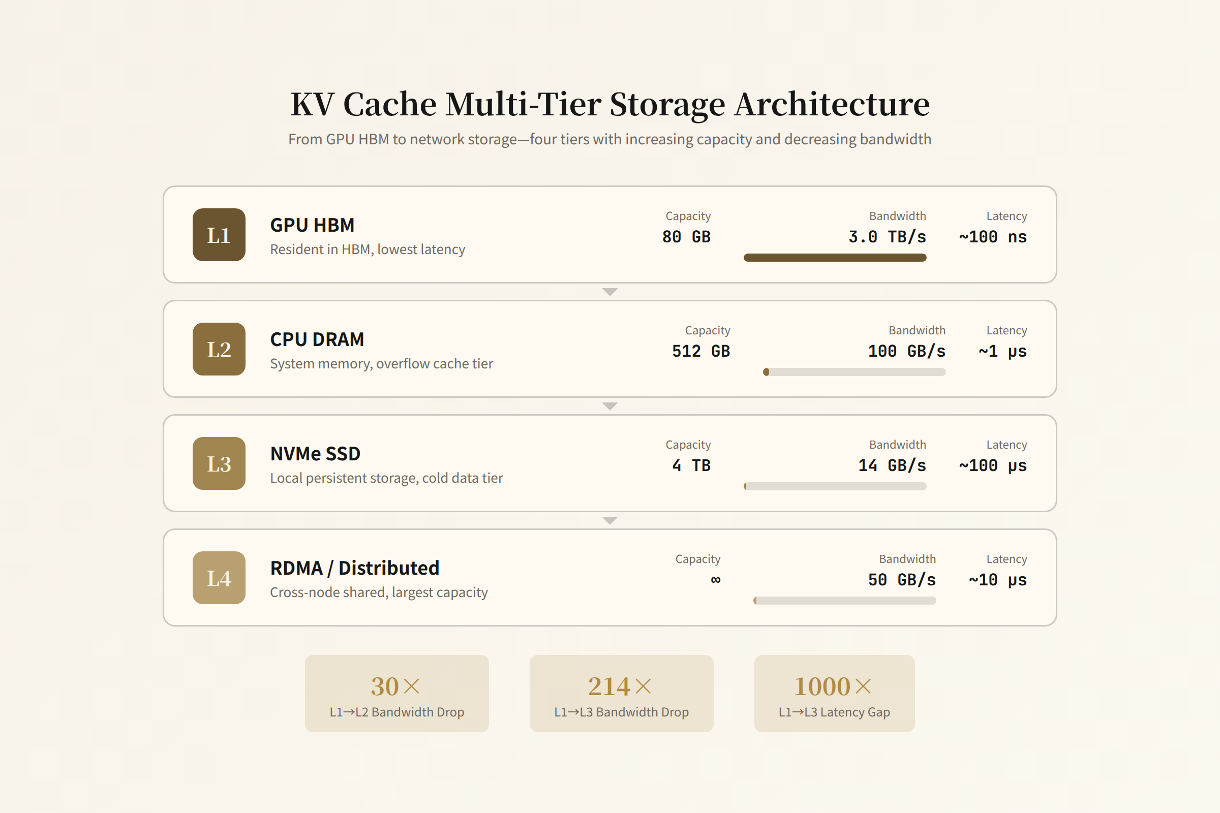
When KV Cache exceeds GPU VRAM, the inference engine starts offloading:
Level 0: GPU HBM (80 GB)
  ↕ Bandwidth: ~3 TB/s (NVLink to other GPUs)

Level 1: CPU DRAM (512 GB–2 TB)
  ↕ Bandwidth: ~100 GB/s (PCIe Gen5)

Level 2: SSD (NVMe, 4–16 TB)
  ↕ Bandwidth: ~14 GB/s (PCIe Gen5 x4)

Level 3: Cross-node RDMA
  ↕ Bandwidth: ~50 GB/s (InfiniBand HDR)
LMCache's approach:
- Prefix sharing: Multiple requests with the same system prompt → share one copy of KV Cache, no duplicate storage
- CPU offloading: What doesn't fit on GPU auto-spills to CPU memory
- Multi-node P2P: Other GPUs/CPUs in the same rack can also lend memory
But each level of offloading carries a latency cost. Reading KV Cache from GPU HBM takes ~0.1ms/layer; from CPU DRAM takes 1–5ms/layer (depending on PCIe bandwidth); from SSD takes 10–50ms/layer. For a 128-layer model, a single decode that needs to fetch all KV Cache from CPU adds 128–640ms of extra latency. This is why KV Cache hit rate has a decisive impact on inference latency.
MoE Expert Dispatch: The Hidden Tax of Communication
MoE Inference Flow
For MoE models, MLP layers are replaced by MoE layers:
Input token → Router Network → Select Top-K Experts → Execute Expert MLP → Weighted merge

Example: DeepSeek V4 has 256 experts, each token activates 8
The key problem: 256 experts' weights total ~350GB (FP16), which doesn't fit on a single GPU. So Expert Parallelism is mandatory — different GPUs hold different expert subsets.
All-to-All Communication
When a token needs an expert that lives on another GPU:
Assume an 8×GPU node with Expert Parallelism = 8 (each GPU holds 32 experts):
- Local hit: GPU 0 needs expert 42 (which it holds) → compute directly
- Cross-GPU fetch: GPU 0 needs expert 200 (held by GPU 3) → send token to GPU 3 via NVLink → GPU 3 computes → result sent back to GPU 0
- All-to-All: Each token may need multiple experts; all GPUs pairwise exchange data
This is All-to-All communication — all GPUs pairwise exchange token data. In an NVLink-connected 8-GPU node: A100: NVLink 3.0, 600 GB/s per GPU H100: NVLink 4.0, 900 GB/s per GPU B200: NVLink 5.0, 1.8 TB/s per GPU
Cross-node All-to-All over InfiniBand is far more expensive: ~50 GB/s bandwidth, 0.5–2ms latency.
DeepEP: Purpose-Built Communication for MoE
In early 2026, DeepSeek open-sourced DeepEP — an All-to-All communication library specifically optimized for MoE Expert Parallelism [5]. The general-purpose NCCL All-to-All primitive isn't optimized for the MoE scenario: MoE dispatch has clear characteristics (each token goes to only Top-K experts, not a full scatter), and communication and computation can be pipelined.
DeepEP's key design decisions:
- Low-precision transmission: Tokens are compressed to FP8 during transfer, halving traffic, then restored to BF16/FP16 for computation on receipt
- Intra-node / inter-node dual mode: Intra-node uses NVLink point-to-point direct transfer; inter-node uses RDMA one-sided writes, avoiding NCCL's collective overhead
- Training + inference dual scenario: High-throughput mode for training (large batches, communication can be well pipelined); low-latency mode for inference (small batches, minimizing single-trip communication latency)
DeepEP reduced MoE layer communication overhead from ~23% to ~12% (intra-node) and from ~75% to ~45% (cross-node) in DeepSeek's own inference scenarios [5]. This transforms large-scale MoE cross-node inference from "theoretically feasible" to "practically deployable."
Communication Overhead Share
In an 8×H100 node with Expert Parallelism = 8:
Single token, single layer MoE computation time:
  Expert MLP computation: ~0.5ms (8 experts in parallel)
  All-to-All communication: ~0.15ms (NVLink, generic NCCL)
  All-to-All communication: ~0.08ms (NVLink, DeepEP optimized)

Communication share (NCCL): 0.15 / (0.5 + 0.15) ≈ 23%
Communication share (DeepEP): 0.08 / (0.5 + 0.08) ≈ 14%
With cross-node Expert Parallelism (InfiniBand):
All-to-All communication: ~1.5ms (generic NCCL)
All-to-All communication: ~0.9ms (DeepEP optimized)

Communication share (NCCL): 1.5 / (0.5 + 1.5) ≈ 75%
Communication share (DeepEP): 0.9 / (0.5 + 0.9) ≈ 64%
Even with DeepEP, cross-node Expert Parallelism still spends 60%+ of time on communication. This is why MoE model inference efficiency depends heavily on network topology — NVLink full connectivity (like NVIDIA SuperPod) is far more efficient than cross-node InfiniBand.
Expert Load Imbalance
Another hidden cost: the Router doesn't assign experts uniformly. Some "popular" experts are selected frequently, while others sit idle. This causes:
- GPUs holding popular experts become bottlenecks (computation queues up)
- GPUs holding cold experts are idle
- Overall GPU utilization drops below 50%
The primary solution today is Expert Parallelism + loss-based load balancing (adding an auxiliary loss during training to penalize uneven assignment). But inference-time load skew persists. This is where observability earns its keep: you need to know the actual call frequency and computation time per expert to decide whether to redistribute experts across GPUs.
Speculative Decoding: Guess and Verify
Kernel-Level Implementation
Speculative Decoding uses a draft model to guess γ tokens, then the target model verifies them in one pass:
1. Draft model generates γ tokens: d₁, d₂, ..., d_γ
2. Target model does one prefill on [original_prompt + d₁...d_γ]
3. Compare target model's predictions t₁...t_γ against draft's d₁...d_γ
4. Keep the matching prefix, discard all draft tokens after the first mismatch
Key optimization: Step 2's prefill can use tree attention — instead of verifying a linear sequence, draft tokens are organized into a tree, and the target model verifies the entire tree in a single forward pass.
From the kernel perspective, tree attention needs a custom attention kernel — because the attention mask is not the standard causal triangle, but a tree structure. Both vLLM and SGLang have implemented their own tree attention kernels.
Engineering Impact of Accept Rate
γ = 5 (draft 5 tokens)
accept_rate = 0.7 (average 3.5 accepted)

Effective tokens per decode:
  Without spec decoding: 1 token / forward pass
  With spec decoding: 3.5 tokens / forward pass

Speedup: 3.5x (theoretical)
Actual speedup: ~2.5x (accounting for draft model overhead and tree attention extra computation)
Accept rate depends on task type:
| Task Type | Accept Rate | Speedup |
|---|---|---|
| Code completion | 75–85% | 3–3.5x |
| Structured output (JSON) | 70–80% | 2.5–3x |
| Conversational replies | 50–65% | 2–2.5x |
| Creative writing | 30–45% | 1.3–1.8x |
For high-accept-rate scenarios like code completion, spec decoding is essentially free acceleration. For creative writing, the draft model overhead may exceed the benefit. The observability imperative: you need to track accept rate by task type to decide whether to enable spec decoding.
MTP: Beyond Speculative Decoding
Speculative Decoding requires a separate draft model — bringing extra VRAM overhead and engineering complexity. DeepSeek V3 proposed MTP (Multi-Token Prediction) as a more elegant alternative [6].
Architecture: One Model, Two Forward Paths
MTP's idea: instead of training a separate draft model, add an MTP head to the main model. The MTP head shares the main model's embedding and most intermediate representations, doing independent prediction only in the last few layers. During training, the MTP head learns to simultaneously predict the next 2–3 tokens (rather than just the standard next token).
Standard model:
  input → Transformer blocks → LM Head → next token

MTP model:
  input → Transformer blocks → LM Head → next token (t₁)
                                → MTP Head 1 → token t₂
                                → MTP Head 2 → token t₃
During inference, the MTP head serves as the speculative decoding draft — but it doesn't need an independent forward pass, since it shares the main model's computation. This is far more efficient than a standalone draft model:
| Approach | Draft Latency | Extra VRAM | Speedup |
|---|---|---|---|
| Standalone draft model (small) | ~30% of target | ~2–5 GB | 2–3x |
| MTP head (shared backbone) | ~5% of target | ~0.5 GB | 2–3x |
| No spec decoding | 0 | 0 | 1x |
Integration with Speculative Decoding
The multiple tokens predicted by the MTP head can be fed directly to the target model for tree attention verification — fully compatible with the standard speculative decoding verification flow. The only difference is the draft source: standalone model vs. shared backbone.
DeepSeek V3's experience shows that MTP + tree attention achieves 2.5–3x speedup in general conversation scenarios, with accept rates 10–15% higher than standalone draft models (because the MTP head shares the main model's semantic understanding) [6].
Observability Implications
MTP introduces new monitoring dimensions:
- MTP prediction accuracy: tracked by position (t₂ accuracy is typically > t₃; the further ahead, the harder)
- MTP head compute overhead share: should be < 10%, otherwise not worth enabling
- MTP + tree attention end-to-end speedup: bucketed by task type
Continuous Batching: The Art of Dynamic Coalescing
Why Not Static Batching
Traditional inference services use static batching: wait for N requests to accumulate → inference together → return together. The problems:
- The last-arriving request determines the entire batch's latency
- Short requests wait for long ones
- Context length variation across requests means padding to max length wastes computation
How Continuous Batching Works
vLLM's continuous batching (also called iteration-level scheduling):
Time T0:
  batch = [req_A (step 15), req_B (step 3), req_C (step 8)]
  All three do one decode forward pass together

Time T1 (after one decode step):
  req_C generated EOS token → done, leaves batch
  req_D just arrived → joins batch
  batch = [req_A (step 16), req_B (step 4), req_D (step 0 prefill)]

Time T2:
  req_A and req_B continue decoding
  req_D finishes prefill, starts decoding
  batch = [req_A (step 17), req_B (step 5), req_D (step 1)]
The batch composition can be dynamically adjusted at every decode step. New requests can join a running batch immediately after prefill — no need to wait for existing requests to finish.
From the kernel perspective, continuous batching's challenge is variable-length batch GEMM/GEMV: each request in the batch has a different context length, different KV Cache size, and different attention sequence length. vLLM solves this with PagedAttention + custom CUDA kernels — each request independently accesses KV Cache through its own block table, with no padding to equal lengths.
Tensor Core: Precision Is Throughput
H100's Tensor Core supports multiple precisions with dramatically different throughput:
| Precision | H100 Peak Throughput | Relative to FP16 Dense | Typical Use |
|---|---|---|---|
| FP64 | 30 TFLOPS | 0.03x | Scientific computing |
| FP32 | 67 TFLOPS | 0.07x | Training |
| TF32 | 495 TFLOPS | 0.5x | Training (accelerated FP32) |
| FP16/BF16 dense | 989 TFLOPS | 1.0x | Inference (standard) |
| FP16/BF16 sparse | 1979 TFLOPS | 2.0x | Inference (structured sparsity) |
| FP8 dense | 1979 TFLOPS | 2.0x | Inference (accelerated) |
| INT4 | ~3958 TFLOPS | 4.0x | Inference (aggressive compression) |
Going from FP16 dense to FP8 dense doubles throughput. Dropping to INT4 gives 4x.
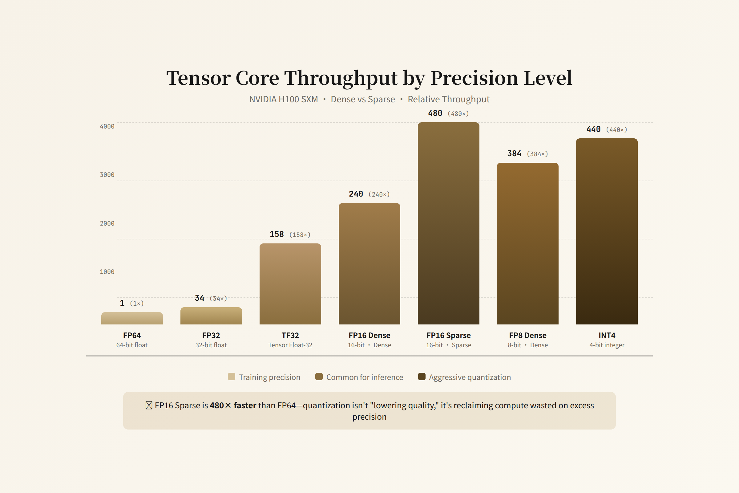
But the cost of lower precision is model quality. FP8 has negligible quality loss in most inference scenarios (<1%) and became the inference standard in 2025. INT4 requires calibration and fine-tuning, with 1–3% quality loss. 2-bit quantization currently works only on specific architectures with larger quality degradation.
Quantization's Impact on Kernels
Different precisions need different CUDA kernels:
- FP16: Standard cuBLAS GEMM kernel
- FP8: H100's FP8 Tensor Core needs specialized kernels (
cublasLtMatmulwith FP8 types) - INT4: Marlin kernel (high-performance GEMM kernel for GPTQ/AWQ quantized models)
vLLM 0.20+ has built-in FP8 inference support, quantizing both model weights and KV Cache. With FP8 enabled, the same GPU doubles throughput and halves VRAM usage — a nearly free optimization.
Blackwell Ultra Architecture: The Next Leap for Inference
All the precision discussion above was based on the Hopper architecture (H100/H200). The NVIDIA Blackwell Ultra architecture (B300/GB300), deployed at scale in 2025-2026, pushes inference performance to new heights. The original B200/GB200 has been superseded by B300/GB300 as the flagship product — B300 delivers 50% higher FP4 throughput than B200 and increases HBM from 192GB to 288GB.
B300 Key Specs
B300 FP4 Tensor Core: ~15 PFLOPS (dense, +50% vs B200)
B300 FP8 Tensor Core: ~7.5 PFLOPS (dense)
B300 BF16 Tensor Core: ~2.25 PFLOPS (dense)
B300 HBM3e bandwidth: 8 TB/s
B300 HBM3e capacity: 288 GB (12-layer stack, B200 is 192GB/8-layer)
B300 typical power: 1400W
B300 process: TSMC 4NP

Arithmetic intensity knee (BF16 dense):
  2250 TFLOPS / 8 TB/s = 281 FLOPS/Byte
  (Comparable to H100's 295 FLOPS/Byte — knee hasn't shifted much)

FP4 knee:
  15000 TFLOPS / 8 TB/s = 1875 FLOPS/Byte
  (Under FP4, the compute-bound threshold is extremely high — most ops remain memory-bound)
The 288GB HBM3e is B300's key improvement for inference. B200's 192GB was already 2.4x H100's 80GB, but long-context Agent workloads (128K+ tokens) can easily consume 100+GB of KV Cache alone. 288GB lets a single card hold larger model KV Cache entirely, reducing cross-GPU offloading. The 12-layer HBM stack (vs B200's 8 layers) also improves bandwidth utilization.
FP4 support is Blackwell's biggest contribution to inference. FP4 compresses both weights and activations to 4-bit, theoretically doubling throughput vs FP8. For precision-insensitive inference scenarios (e.g., candidate generation, batch prefill), FP4 can dramatically reduce cost. But FP4 requires calibration and fine-grained block-wise scaling — engineering complexity is higher than FP8.
GB300 NVL72: Rack-Scale Inference Supercomputer
GB300 NVL72 is NVIDIA's flagship inference deployment form factor — 72 B300 GPUs + 36 Grace CPUs in a single rack connected via NVLink:
- Total FP4 compute: ~1.08 EFLOPS (72 × 15 PFLOPS)
- Total HBM capacity: ~20.7 TB (72 × 288GB)
- NVLink domain bandwidth: 130 TB/s
- Pricing: ~$3.7-5M per rack
NVL72's significance: 72 GPUs form a single compute domain — no cross-node communication needed to run a complete MoE model. This structurally improves MoE inference All-to-All communication overhead — from ~50 GB/s on cross-node InfiniBand to ~1.8 TB/s per GPU within the NVLink domain.
Transformer Engine Generation 2
Blackwell's companion Transformer Engine 2 (TE2) provides deep software-level optimization:
- Automatic precision selection: per-layer auto-determination of FP4/FP8/BF16, finding the optimal balance between precision and speed
- Native FP4 attention: attention computation entirely in FP4 precision (requires FA4-level kernel support)
- Mixed-precision pipeline: prefill in high precision, decode in low precision, auto-switched by TE2
Energy Efficiency Leap
NVIDIA official data: Blackwell inference delivers ~50x more tokens per watt than H100. This number breaks down as: ~5x from FP4 vs FP16 precision improvement, ~3x from architecture changes (larger SRAM, more efficient Tensor Core), ~3x from HBM3e bandwidth improvement and 288GB capacity. Combined, these reach 50x on specific workloads.
Important: B300 specs don't override H100 data. The two architectures coexist in 2026: H100 for existing inference clusters, B300 for new high-density deployments. Observability tools must cover both architecture generations — don't assume all GPUs are Blackwell.
The Three Layers of Observability
At this point, we've broken down every phase of the inference engine from Prefill to Decode, from Attention to MoE Dispatch, down to the kernel level. But "can be decomposed" ≠ "can be observed" — you need tools to actually measure these processes. Inference engine observability naturally splits into three layers, echoing the series' "three blind spots" theme.
Layer 1: Request-Level
The most basic observability: per-request latency and throughput. vLLM's exposed Prometheus metrics represent this layer:
vllm:num_requests_running      — Number of running requests
vllm:num_requests_waiting      — Number of queued requests
vllm:gpu_cache_usage_perc      — KV Cache usage ratio
vllm:num_preemption            — Number of preemptions due to VRAM exhaustion
vllm:e2e_request_latency_seconds — End-to-end latency
vllm:time_to_first_token_seconds — TTFT (time to first token)
vllm:time_per_output_token_seconds — TPOT (time per output token)
gpu_cache_usage_perc is the single most critical metric. When it approaches 100%, new decode requests must wait for existing requests to release KV Cache space — manifesting as latency spikes. But this metric only tells you "it's full," not "why it's full."
Missing dimensions in request-level observability:
- TTFT decomposition: Out of 320ms TTFT, how long was queue wait? How long was prefill compute? How much was network latency? vLLM's metrics don't break this down.
- Tail latency attribution: Why is P99 latency 5× higher than P50? Was a particular request extra long, or did a preemption happen at some moment?
- Cross-request prefix sharing detection: How many requests share the same system prompt? Is the sharing rate 10% or 80%? This directly affects actual KV Cache occupancy.
Layer 2: Kernel-Level
When you need to explain "why is TTFT 320ms," you need a kernel-level timeline.
NVIDIA Nsight Systems provides a global timeline of GPU execution:
- Start/end time of every CUDA kernel
- CPU-GPU data transfers
- Memory allocation/deallocation
- NCCL communication operations
- CUDA stream parallel execution
This is the first step in locating inference engine bottlenecks — find the widest section on the timeline, or gaps where the GPU is waiting on CPU or network.
NVIDIA Nsight Compute performs deep analysis on a single kernel:
- Tensor Core utilization
- HBM read/write bandwidth utilization
- SRAM usage
- Occupancy (ratio of active warps)
- Roofline analysis (arithmetic intensity vs. actual throughput)
Nsight Systems tells you "which kernel is slow"; Nsight Compute tells you "why it's slow." Together, they form the standard GPU profiling workflow.
Graphsignal adds finer-grained profiling on top of vLLM metrics:
- Per-step prefill/decode time breakdown
- LLM generation tracing (per-token latency distribution)
- Tool-call-level timing analysis
- Continuous high-resolution timeline (not sampled)
Layer 3: Semantic-Level
Request-level and kernel-level are the territory of traditional GPU profiling. But inference engines have a unique set of "semantic metrics" — they aren't generic GPU metrics, but specific to LLM inference:
MoE Expert load distribution monitoring: Across 256 experts, which ones are over-called? How severe is the imbalance? If the Top-10 experts' call frequency is 50× that of the Bottom-10, it means the Router's load-balancing training was insufficient, or inference-time token distribution has drifted from training. This metric is almost entirely missing from existing tools — vLLM doesn't expose per-expert call statistics, and Nsight can't see the semantic concept of experts.
KV Cache lifecycle tracking: The complete history of a KV block from allocation to eviction. Allocated → hit (read by attention) → possibly offloaded to CPU → possibly evicted (under VRAM pressure) → possibly recomputed (when the request needs it again). Existing tools only tell you current gpu_cache_usage_perc; they don't show you the flow patterns of KV blocks.
Spec Decoding accept rate bucketed by task type: An overall accept rate of 70% might mask "code completion 85%, creative writing 35%." You need per-request-type (prompt classification, routing info) accept rate buckets to make precise per-request enable/disable decisions.
Prompt Caching hit rate: Prefix match rate vs. full match rate. Prefix match rate = matched prefix tokens / total input tokens. Full match rate = requests with a prefix hit / total requests. The two metrics measure efficiency at different levels.
The common characteristic of these semantic-level metrics: they don't exist in GPU performance counters; they must be actively exposed by the inference engine itself. This means the engine needs instrumentation — not in CUDA kernels, but in the scheduler, Router, and KV Cache manager logic.
Closing the Loop Between Layers
The three layers aren't isolated — they need to cross-reference each other to form complete observability:
Request-level: TTFT = 320ms (know "it's slow")
  ↓ drill down
Kernel-level: Flash Attention kernel takes 160ms (know "where it's slow")
  ↓ drill down
Semantic-level: This request's context length is 35K, in the top 1%
  (know "why it's slow")

  ↓ attribute to series theme
Inference engine metrics → token cost attribution (Layer 1 blind spot: Cost)
Inference quality signals → Agent drift detection (Layer 3 blind spot: Agent decisions)
Inference engine observability ultimately serves the other two layers of the series: cost and Agent decisions. Without kernel-level drill-down, cost attribution is limited to crude "GPU-hours ÷ token count" averaging; without semantic-level tracking, Agent drift detection can only do after-the-fact analysis on output text, blind to anomaly signals inside the inference engine.
Auto-Tuning: From Manual to AI-Autonomous
The Curse of Dimensionality in Configuration Space
The inference engine's configuration parameter space is enormous:
| Parameter | Range | Performance Impact |
|---|---|---|
| Batch size | 8–512 | Throughput vs. latency |
| KV cache budget | 0.5–80 GB | Concurrency vs. context length |
| Spec decoding gamma | 0–8 | Speedup vs. extra compute |
| Quantization level | FP16/FP8/INT4 | Throughput vs. quality |
| Tensor parallel size | 1–8 | Throughput vs. GPU utilization |
| Expert parallel size | 1–256 | Communication overhead vs. VRAM |
| Prefill chunk size | 512–8192 | TTFT vs. compute efficiency |
These parameters are coupled — batch size affects KV Cache consumption, quantization affects expert load distribution, spec decoding gamma affects effective batch size. Human tuning can only explore a tiny subset of this space.
Current Automation Directions
Graphsignal's continuous profiling mode: Continuously collects kernel-level profiling data and uses statistical models to identify "performance anomalies" — e.g., a batch where the attention kernel is 3× slower than the historical mean. This is essentially anomaly detection, not yet auto-remediation.
vLLM's adaptive batching: vLLM's scheduler dynamically adjusts batch composition based on current KV Cache usage — preempting low-priority requests when memory is tight, admitting more requests when memory is plentiful. But this is single-parameter adaptation, not global optimization.
NVIDIA AVO: AI-Autonomous Kernel Generation
The most radical direction comes from NVIDIA itself — AVO (Agentic Variation Operator) [7]. AVO is an AI agent that takes an initial GPU kernel implementation and automatically generates variants, compiles, benchmarks on real GPUs, analyzes bottlenecks, and generates improved variants — in a loop.
Results on attention kernels: AVO-generated kernels are 10.5% faster than Flash Attention 4's hand-written kernel [7]. The optimizations AVO discovered include: automatically finding better tile sizes, auto-tuning warp specialization strategies, automatically discovering deeper asynchronous pipeline depths — directions that would take human experts weeks to explore.
The significance here goes far beyond "10% faster" — it marks kernel optimization transitioning from human craft to AI search space. The role of observability fundamentally shifts as a result:
Traditional mode:
  Tools → Human engineer examines data → Human diagnoses bottleneck → Human modifies code

AVO mode:
  Tools → AI agent examines data → AI generates variants → AI benchmarks → AI selects the best
  Humans only need to define "what good looks like"
Observability shifts from "helping humans see problems" to "helping AI see problems." Data formats, sampling frequencies, and feedback latency all need redesign — AI agents need programmatic, structured performance data, not human-facing visualization dashboards.
Closed-Loop Architecture
Integrating the above directions, the closed-loop architecture for inference engine auto-tuning is:
- Deploy inference service (initial configuration)
- Three-layer telemetry continuous collection
- Request-level: latency distribution, throughput, preemptions
- Kernel-level: per-kernel timing, bandwidth utilization
- Semantic-level: expert distribution, KV lifecycle, accept rate by task type
- Bottleneck analysis (AI-assisted)
- "MoE expert 42 call rate is 8× mean → consider expert duplication"
- "decode accept rate for JSON = 35% → disable spec decoding for creative tasks"
- "FA kernel bandwidth utilization = 60% → AVO tries better tile size"
- Auto-tune + kernel optimization
- Config: batch, cache, spec on/off
- Kernel variants: AVO generates and benchmarks
- Canary deployment + A/B verification
- Return to step 2, continuous loop
This isn't hypothetical — every individual link has a 2026 product doing it. What's missing is connecting them into an automated closed loop, rather than requiring human engineers to make manual decisions at each handoff.
The Inference Observability Matrix: A Global View
The preceding chapters analyzed the inference engine from individual technical angles — Prefill/Decode, KV Cache, MoE, Spec Decoding. The sections below unify them into a single observability matrix grounded in real-world inference operations — one that any inference SRE or platform engineer can deploy directly.
The Observability Matrix
Grouped by inference phase, each table lists only key metrics and baselines. Tools and instrumentation methods are covered in the three-layer telemetry architecture below.
Prefill / Decode
| Point | Metric | Healthy Baseline |
|---|---|---|
| TTFT (time to first token) | P95 TTFT (ms) | < 500ms (32K input) |
| Prefill throughput | tokens/sec | > 5,000 (H100 FP16) |
| TPOT (time per output token) | P95 TPOT (ms) | < 30ms (single request) |
| Decode batch size | running_batch_size | > 16 (effective continuous batching) |
KV Cache
| Point | Metric | Healthy Baseline |
|---|---|---|
| VRAM utilization | gpu_cache_usage_perc | < 85% |
| Preemption count | num_preemption | 0 (> 0 means VRAM shortage) |
| Prefix cache hit rate | prefix_cache_hit_rate | > 60% (Agent workloads) |
| Eviction rate | kv_cache_eviction_rate | < 5% |
MoE / Spec Decoding
| Point | Metric | Healthy Baseline |
|---|---|---|
| Expert load distribution | expert_load_cv | < 0.3 |
| All-to-All communication | all_to_all_latency_ms | < 25% of total inference time |
| Spec decoding accept rate | accept_rate_by_task | Code > 70%, Chat > 50% |
| Effective speedup | effective_speedup | > 1.5x |
GPU Hardware
| Point | Metric | Healthy Baseline |
|---|---|---|
| Tensor Core utilization | tensor_core_util | Prefill > 50%, Decode < 5% |
| HBM bandwidth utilization | hbm_bandwidth_util | Decode > 80% (memory-bound) |
| Attention kernel time share | attention_time_fraction | Prefill 30-40%, Decode 15-25% |
| GPU power draw | power_draw (W) | < 90% TDP |
Instrumentation: Three-Layer Telemetry Architecture
-
Layer 1: Standard Metrics (low cost, always-on)
- vLLM Prometheus exporter (every 15s): TTFT/TPOT distribution, KV Cache usage, batch size, preemption count
- DCGM exporter (every 10s): GPU utilization/power/temp, HBM bandwidth/VRAM, Tensor Core utilization
- API gateway metrics: request latency distribution, error rate (429/500), throughput
-
Layer 2: Distributed Tracing (medium cost, sampled)
- OpenTelemetry + OpenInference spans: one span per LLM call, carrying model, token_count, cost, cached_tokens
- Agent step → LLM call → tool call complete call chain
- Sampling rate: production 1-5%, debug 100%
-
Layer 3: GPU Kernel Profiling (high cost, on-demand)
- Nsight Systems timeline: per-kernel execution time, CPU-GPU transfer, NCCL communication
- Nsight Compute roofline: Tensor Core utilization, HBM read/write bandwidth, occupancy
- Trigger: automatically when Layer 1/2 detects anomalies
Closing the Loop: From Metrics to Action
| Observed Anomaly | Root-Cause Analysis Path | Auto/Manual Response |
|---|---|---|
| TTFT P95 sudden spike | KV Cache usage → prefill queuing → GPU utilization | Scale prefill instances (PD disaggregation) |
| TPOT P95 gradual rise | Batch size → KV Cache eviction rate → HBM bandwidth | Reduce batch or scale decode instances |
| Spec decoding speedup degradation | accept_rate bucketed by task type → which task is dragging it down | Disable spec decoding for low-accept-rate task types |
| MoE expert load imbalance | expert_load_cv → which experts are hot/cold | Reassign experts across GPUs or add load-balancing loss |
| GPU power abnormally low | Tensor Core utilization → decode ratio → batch size | Normal (decode is memory-bound) or coalesce more requests into batch |
Series Callback
The inference observability matrix is not isolated — its TTFT/TPOT anomalies trigger DD1's cost alerts, and its inference quality signals trigger DD3's Agent drift detection. Observability data from all three blind spots ultimately needs to be correlated under a unified trace ID.
Tool Landscape and Challenges
Current state: vLLM's Prometheus exporter is the de facto standard for inference engine metrics — TTFT, TPOT, KV Cache usage, preemption counts and other core metrics are widely adopted. NVIDIA DCGM + Nsight Systems/Nsight Compute is the standard GPU profiling stack: DCGM for continuous hardware metric collection, Nsight Systems for kernel-level timelines, Nsight Compute for single-kernel roofline analysis. Graphsignal does continuous profiling, breaking inference into fine-grained prefill/decode/KV Cache timelines, but with limited coverage (supported inference engines and model architectures are still insufficient). SGLang's built-in metrics are rapidly maturing. However, kernel-level profiling (Nsight) still requires expert manual operation — run the profiler, export the timeline, visually analyze kernel shares — an extremely high bar.
Challenges:
-
The barrier to kernel-level profiling is too high. An Nsight Systems timeline contains thousands of kernel calls, each with start/end/duration/SM utilization fields. Interpreting this data requires deep GPU architecture knowledge — what is WGMMA, what is occupancy, why is a GEMM kernel's Tensor Core utilization only 40%. This is a black box for most SREs.
-
No standardized correlation between inference engine metrics and Agent traces. vLLM's request_id and Langfuse's trace_id don't auto-align. When you see an Agent step's latency spike in Langfuse and want to drill into vLLM's engine state at that moment, you can only correlate by timestamp — which is nearly impossible under high concurrency.
-
Key metrics like MoE expert distribution and spec decoding accept rate aren't exposed in most engines' default metrics. vLLM doesn't output per-expert call frequency by default; SGLang doesn't include accept-rate-by-task-type bucketing in standard metrics. These semantic-level metrics require the engine to instrument itself — not in CUDA kernels, but in the scheduler and Router logic.
-
Blackwell architecture features require new profiling methodologies. FP4 precision roofline analysis differs from FP16/FP8; TMEM (Tensor Memory) read/write patterns can't be modeled with SRAM analytics; 2-CTA MMA's dual thread array cooperation needs new performance counters. DCGM support for Blackwell is still catching up.
Requirements for the tooling ecosystem:
- Automated kernel bottleneck diagnosis — instead of requiring experts to read Nsight timelines, tools should automatically identify "Flash Attention takes 35% of prefill, GEMM takes 50%, MLP down-projection Tensor Core utilization is low" and suggest optimizations
- Automatic correlation between inference engine traces and application-layer traces — shared request_id (or automatic trace context propagation via OTel context), enabling one-click drill-down from Langfuse's Agent step span to vLLM's engine metrics
- Pluggable metrics exporter architecture — allowing semantic metrics like MoE expert distribution and spec decoding accept rate to be exposed via plugins, rather than waiting for official engine support
Verdict: From Black Box to Glass Box
Inference engine observability is evolving from "good enough metrics" to "full kernel-level transparency." The end state isn't a monitoring dashboard — it's a self-optimizing system where the inference engine perceives its own performance bottlenecks in real time and auto-tunes its configuration, even auto-generating better kernels.
Whoever gets there first defines the standard for next-generation inference infrastructure. vLLM has the open-source ecosystem advantage; NVIDIA has hardware depth and AI-autonomous optimization capabilities like AVO; but third-party tools (Graphsignal, Langfuse, Phoenix) have a shot at becoming the unified observation layer across engines and hardware.
The inference engine's journey from black box to glass box means kernel-level telemetry will likely become standard for inference services within 12 months. When every millisecond of GPU time is precisely measured and optimized, "inference cost" transforms from an accounting problem into an engineering problem — and engineering problems are solvable.
But there's a deeper shift underway: when AI agents like AVO can generate better kernels faster than humans, the ultimate consumer of observability tools is no longer the human engineer, but the AI itself. Designing performance feedback channels for AI — structured, high-frequency, programmatic — may be the true competitive moat for the next generation of inference infrastructure.
References
[1] Shah, Dao et al., "FlashAttention-3: Fast and Accurate Attention with Asynchrony and Low-precision", 2024. arXiv:2407.08691.
[2] AMD / SGLang, "Prefill-Decode Disaggregation on AMD GPU", 2025. See AMD ROCm blog and SGLang docs. Chatbot scenario 95th percentile Goodput improvement 6.9x, decode-heavy scenario 2.2x. The 6.4x cited in the original source is a weighted average across scenarios.
[3] Dao, Haziza et al., "FlashAttention-4: Algorithm-Kernel Co-Design for Blackwell", 2026. arXiv:2603.05451. B200 BF16 reaches 1613 TFLOPS (71% utilization), implemented using CuTe-DSL.
[4] DeepSeek-AI, "FlashMLA: Efficient MLA Decoding Kernels for Hopper GPUs", 2026. See github.com/deepseek-ai/FlashMLA. MLA compresses KV Cache by 93% (10 GB → 0.67 GB / 1000 tokens), 3000 GB/s bandwidth and 580 TFLOPS on H800.
[5] DeepSeek-AI, "DeepEP: Efficient All-to-All Communication for MoE Expert Parallelism", 2026. See github.com/deepseek-ai/DeepEP. Supports FP8 transmission, intra-node/inter-node dual mode.
[6] DeepSeek-AI, "DeepSeek-V3 Technical Report", 2025. MTP head design: predicts 2–3 tokens at once, shares main model backbone, serves as spec decoding draft during inference. Accept rate 10–15% higher than standalone draft models.
[7] NVIDIA, "Agentic Variation Operator (AVO): AI-Generated GPU Kernels", 2026. AVO-auto-generated attention kernels are 10.5% faster than FA4's hand-written kernel. See NVIDIA Research.
[8] NVIDIA, "Blackwell B200 Architecture Whitepaper", 2024. FP4 Tensor Core ~20 PFLOPS, HBM3e 8 TB/s, tokens per watt 50× Hopper (official data).
The next Deep Dive focuses on Agent decision path observability — when an AI Agent goes off track at step 7 of a 20-step task, why traditional monitoring is completely blind to it, and how emerging Agent observability tools are trying to fill the gap.