In February 2026, Jose M. Castro — a Distinguished Fiber Optic R&D Engineer at Panduit — presented a short but precise report at the IEEE 802.3 E4AI workshop. Its title: "Optical Shuffle Architectures for Large AI Networks." The key number inside: in a 32,768-GPU cluster, Optical Shuffle cuts total transceiver count by roughly 33% while reducing spine switches from 256 to 64 — a 4× gap.
Two months later, AWS published RNG (Resilient Network Graphs), replacing fat-tree topology with random graphs and eliminating 69% of routers. RNG reimagines the architecture. Castro reimagines the fiber.
At first glance, the two efforts seem unrelated — one changes topology, the other changes cabling. But together they point to the same conclusion: the network cost bottleneck for AI clusters is not in switching silicon. It's in fiber and transceivers. Whoever solves the physical layer first gets the ticket to the next scale-up.
This article does three things: breaks down Optical Shuffle's technical mechanism and quantified gains, analyzes how it complements (and conflicts with) RNG, and evaluates what MCF (multicore fiber) and HCF (hollow-core fiber) mean for AI networking over the longer term.
The Problem: Transceivers Are the Real Cost Center
Consider the numbers.
An 8,192-GPU AI cluster typically deploys 1,024 nodes (8 GPUs each), 128 leaf switches, and 64 spine switches. All switches are 512-port. Standard fat-tree (spine-leaf) covers this comfortably.
But at 32,768 GPUs?
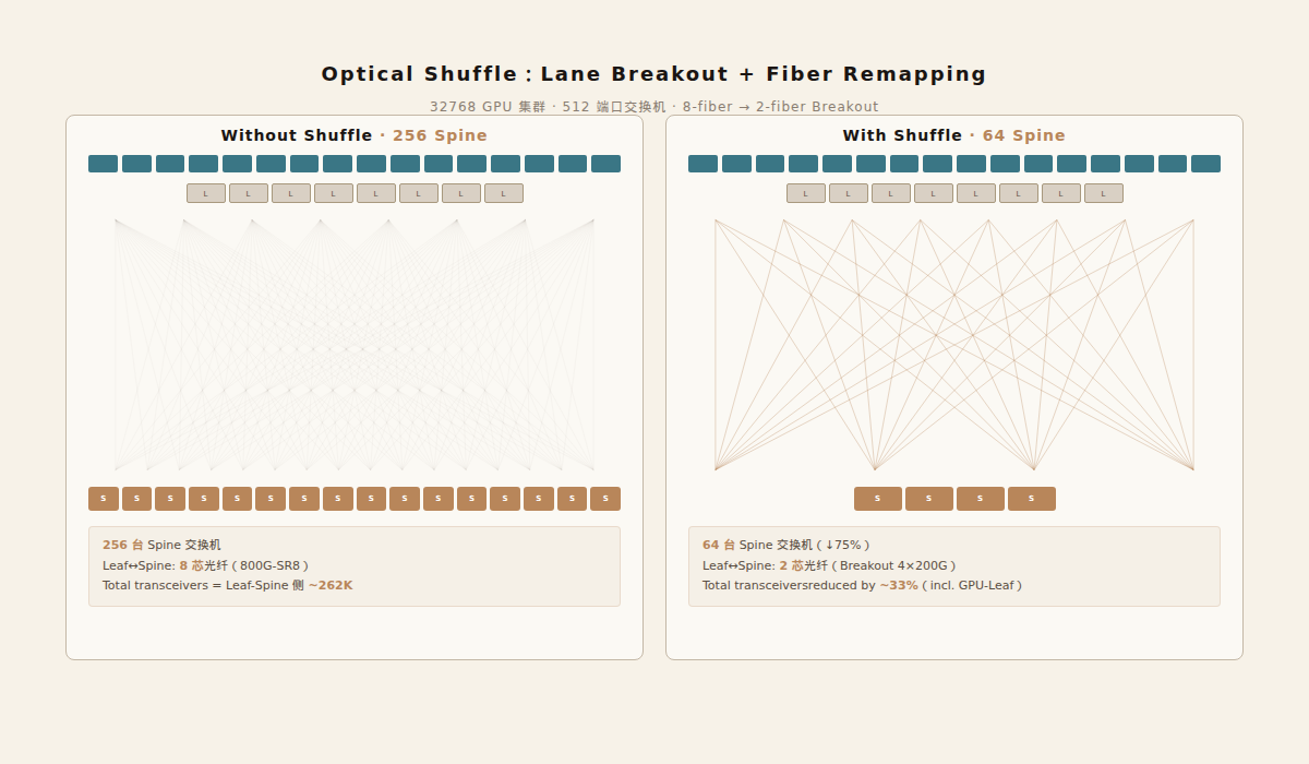
4,096 nodes, four copies of the 8K cluster — 64 PODs. Using the same 512-port switches, spine count jumps from 64 to 256. Leaves go from 128 to 512. Each leaf needs a pair of optical transceivers for every spine connection.
Total transceiver count ≈ leaf count × uplinks per leaf + GPU-to-leaf connections. Rough calculation:
- 512 leaves × 256 spines each = 131,072 transceivers (leaf-spine side)
- 32,768 GPUs connecting at 400G to leaves = another large batch
- Total: 150,000–200,000 transceivers for a 32K-GPU cluster
An 800G OSFP transceiver currently costs $500–$800. 150,000 units = $75M–$120M. The switches themselves are almost an afterthought — a 512-port 800G switch runs about $50K–$100K; 256 spines cost $13M–$25M.
Transceivers cost 3–5× what the switches cost. This ratio existed at 400G and amplifies at 800G/1.6T — more fibers, more precise optics, higher-power DSPs per lane.
Castro's question was precise: without touching topology or routing protocols, just reorganizing how fibers connect, how many transceivers can you eliminate?
How Optical Shuffle Works: Lane Breakout + Fiber Remapping
Lane Breakout: One Thick Pipe Becomes Four Thin Ones
Modern 800G transceivers (e.g., 800G-SR8) use 8 fibers in parallel — 8 channels, each running 100G. The module end is an 8-fiber MPO connector. The far-end switch has a matching 8-fiber MPO. A single 8-fiber jumper connects them, fiber for fiber.
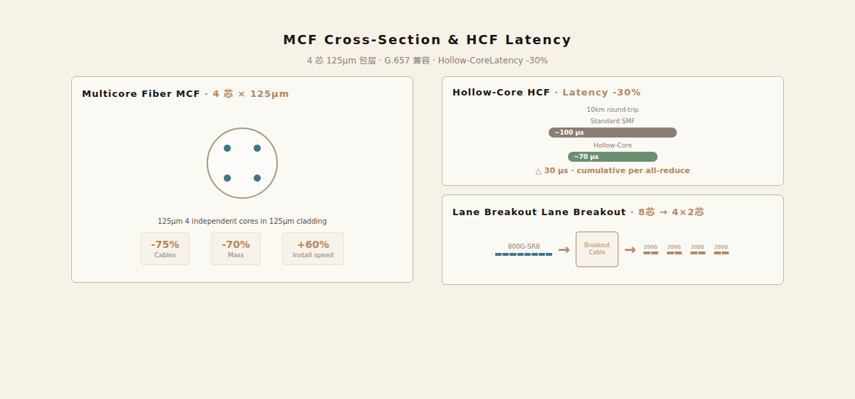
Lane Breakout does something simple: split one 8-fiber MPO into 4 groups of 2 fibers (one TX, one RX each). Instead of connecting to one far-end module, the 8 fibers from a single 800G-SR8 module distribute to 4 different far-end modules, each running 200G over 2 fibers.
Physically this is just a breakout cable — one end is 8-fiber MPO, the other is 4× LC duplex connectors. Cost: $10–$30. Passive, no power.
Shuffle: Reorganize Which Signals Go Where
Breakout alone just splits "one into four." The shuffle step is where the real work happens: re-mapping at the fiber layer which signals are delivered to which destination.
In a standard fat-tree, one leaf's uplink ports distribute to 64 spines, each spine using 8 fibers (one 800G link). Castro's proposal: breakout the leaf uplink into 2-fiber groups, each routed through a shuffle panel to a different spine.
Result: each spine no longer needs a full 800G port (8 fibers) — just one 200G channel (2 fibers). The same 512-port switch now serves 4× as many leaf connections per port.
Quantified Gains
8,192-GPU cluster:
| Without Shuffle | With Shuffle | |
|---|---|---|
| GPUs | 8,192 | 8,192 |
| Nodes | 1,024 | 1,024 |
| Leaves | 128 | 128 |
| Spines | 64 | 64 |
| Leaf-Spine connection | 8-fiber | 2-fiber |
| Spine port utilization | 1 leaf per port | 4 leaves per port |
At 8K scale, spine count stays the same (64), but each spine's port efficiency increases 4×.
32,768-GPU cluster:
| Without Shuffle | With Shuffle | |
|---|---|---|
| GPUs | 32,768 | 32,768 |
| Nodes | 4,096 | 4,096 |
| PODs | 64 | 64 |
| Leaves | 512 | 512 |
| Spines | 256 | 64 |
Spines drop from 256 to 64 — a 4× reduction. This eliminates 192 spine switches and all their transceivers.
Total transceiver reduction (including GPU-leaf side): ~33%.
Why It Works
The key insight is that AI training traffic patterns differ from general data center traffic.
General-purpose DCs need fat-tree full-mesh — every leaf to every spine at full bandwidth (800G), because traffic is unpredictable. But AI training is highly structured: in all-reduce operations, each leaf exchanges gradient data with every other leaf, but the per-exchange bandwidth doesn't always require a full 800G pipe. Sufficiently many 200G channels (ECMP multipath) can handle the load.
Lane Breakout converts 1×800G link into 4×200G links. Total bandwidth stays 800G, but connection count quadruples. For AI training's all-reduce pattern, more paths at finer granularity beat fewer fatter pipes — better load balancing, fewer hash collisions.
This is the mathematical foundation: not less bandwidth, but better-distributed bandwidth, letting the same switching silicon serve more connections.
RNG vs. Optical Shuffle: Changing Topology vs. Changing Fiber
Now put Castro and AWS side by side.
Orthogonal Dimensions
| RNG (AWS) | Optical Shuffle (Castro/Panduit) | |
|---|---|---|
| What changes | Network topology — fat-tree → random graph | Fiber connection method — breakout + remap |
| Core mechanism | Spraypoint routing + ShuffleBox cabling | Lane breakout cable + shuffle panel |
| Target | Switches and routing | Transceivers and fiber |
| Cost saving source | Routers -69% | Transceivers -33%, Spines -75% |
| Prerequisite | Must replace topology and routing protocol | No topology change — operates within fat-tree |
| Use case | Multi-tenant general compute | AI GPU training clusters |
| Engineering risk | Must rebuild ops toolchain | Fiber cabling changes, minor ops adjustments |
| Compatibility | Replaces fat-tree | Coexists with fat-tree |
The critical distinction: RNG is a replacement. Shuffle is an optimization. RNG says "fat-trees are wrong." Shuffle says "fat-tree fibers aren't routed efficiently." They're not contradictory — in theory they can be stacked.
Can They Be Combined?
Theoretically yes, with a constraint: RNG's ShuffleBox and Shuffle's breakout panel compete for the same fiber endpoints at the physical layer.
RNG's ShuffleBox is a passive fiber cross-connect — scattering router uplinks to random remote endpoints. Castro's shuffle panel is also passive — splitting 8-fiber into 4×2-fiber and remapping. If chained in series, signals pass through two panels, and connector losses accumulate.
RNG's paper already discusses the optical-loss constraint: paths exceeding 7 connectors are pruned. Adding a shuffle panel means +2 connectors. If RNG's ShuffleBox already accounts for 4–6 connectors, stacking one more panel may exceed the transceiver's power budget.
Combining them is feasible but has a physical ceiling — dependent on specific transceiver power budgets and link lengths. Short-reach (<100m OM4 multimode) has margin for stacking. Long-reach (>500m single-mode) is tighter — you may have to choose one.
Combined Impact on Transceiver Cost
RNG eliminates 69% of switches, which removes most of their transceivers. But each remaining router still needs optical modules. The total transceiver reduction depends on the router reduction ratio plus the per-router port density change.
Shuffle reduces transceivers per link — not fewer switches, but fewer transceivers per switch serving the same connectivity. The 33% reduction is a direct cost cut.
If both are combined: RNG first eliminates 69% of switches (cutting ~50–60% of transceivers — inter-router links shrink dramatically, but GPU-leaf links stay). Then Shuffle cuts another 33% from the remainder. Total transceiver reduction: roughly 65–70%.
But this is theoretical. No combined RNG + Shuffle deployment exists in public literature.
The Two Longer Roads: MCF and HCF
Castro's second presentation at the same workshop looked further ahead — not just how to connect fibers, but how the fibers themselves are changing.
MCF (Multicore Fiber): One Strand, Four Paths
MCF isn't a new concept — embed 4 independent cores within a standard 125µm cladding, each carrying a separate optical signal. Physical outer diameter matches standard G.657 fiber, fitting the same conduits and connectors.
Castro's design parameters:
| Parameter | Value |
|---|---|
| Core count | 4 |
| Cladding diameter | 125 µm |
| Coating diameter | 200/250 µm |
| Attenuation | < 0.4 dB/km (1310nm), < 0.20 dB/km (1550nm) |
| Mode field diameter | 8.6–9.2 µm |
| Crosstalk | ≤ -40 dB (@1310nm or @1550nm, 10km) |
| Bending loss | ≈ conventional G.657.A1 |
Key signal: G.657 compatible. MCF can be deployed in existing fiber conduits without infrastructure changes. Connectors, splicing machines, and test equipment need adaptation, but the physical pathway remains the same.
At OFC 2026 (March 2026), Corning launched an MCF product line for AI data centers with concrete benefit numbers:
- Cable and connector count reduced by 75%
- Cable mass reduced by 70%
- Installation speed improved by 60%
These numbers matter because AI data center fiber counts are exploding. AFL Hyperscale's analysis: AI data centers need 10× more fiber than traditional data centers. A 32,768-GPU cluster needs tens of thousands of fiber jumpers for GPU-to-leaf alone, plus tens of thousands more for leaf-to-spine. Without density improvements, fiber management becomes a physical bottleneck — not bandwidth, but sheer cable volume.
MCF's hidden benefit: it can extend 400G-PAM4 reach at 1310nm. ITU's analysis shows standard SMF limits 400G-PAM4 under CWDM to <1km due to chromatic dispersion, but MCF with PSM (parallel single-mode), each core independently running a wavelength near 1310nm, extends effective 400G reach to ~3km — exactly covering campus-scale AI data center inter-building links.
MCF's costs:
- Splicing requires rotational alignment — 4 cores must be precisely matched. Standard fusion splicers can't do this; specialized equipment needed. Field installation time increases.
- Fan-in/fan-out devices are mandatory for interfacing MCF with conventional single-core optics, adding ~0.3–0.5 dB insertion loss per device.
- Fault isolation is more complex — one core may fail while three survive. Test equipment must distinguish cores.
- Standardization is still in progress — ITU-T G.650.x series is being supplemented with MCF test methods and parameter definitions.
Judgment: MCF is not an optional future — it's a necessary one. When AI clusters move from 10K to 100K GPUs, fiber density becomes a physical hard constraint. MCF's 4× density improvement is the only mature path currently available. The costs are primarily operational — tool and process adaptation. These are far cheaper than building new physical space for more cables.
HCF (Hollow-Core Fiber): Light Travels Faster in Air
HCF's principle is different — optical signals propagate through air-filled channels inside the fiber rather than through glass. Light travels ~30% faster in air than in silica glass, directly reducing propagation delay.
Who cares most about 30% latency reduction? Cross-building, cross-campus distributed AI training.
Round-trip latency comparison:
| Link length | Standard SMF round-trip | HCF round-trip | Delta |
|---|---|---|---|
| 2 km | ~20 µs | ~14 µs | 6 µs |
| 10 km | ~100 µs | ~70 µs | 30 µs |
| 40 km | ~400 µs | ~280 µs | 120 µs |
In large-model training, every all-reduce operation requires all GPUs to synchronize at microsecond granularity. If cross-building link round-trip differs by 30 µs (10km scenario), the difference accumulates with each iteration. At 100K-GPU scale with hundreds of cross-cluster synchronizations per second, the latency gap significantly impacts training efficiency.
But HCF's costs are much higher than MCF's:
- Manufacturing is fundamentally different from conventional fiber — precise internal microstructure control required. Low current production volume, high cost.
- Splicing carries risk — imprecise heat control can collapse the hollow core structure.
- Interfaces with conventional fiber need specialized components — glass-to-air boundaries introduce reflections.
- Ribbon HCF and high-core-count HCF cables are not yet commercially available.
- Microsoft has deployed HCF in Azure, but at limited scale.
AFL Hyperscale's assessment is clear-eyed: "Neither technology is expected to broadly replace conventional SMF. Adoption will depend on whether the performance advantages justify both the operational complexity and the TCO."
Judgment: HCF's applicable scenario is very narrow — limited to cross-building/cross-campus AI cluster interconnects (Scale-Across layer). In Scale-Out (intra-data-center) and Scale-Up (intra-rack) layers, the latency difference isn't large enough to justify HCF's operational complexity. But at 10km+ distributed training scenarios, 30% latency reduction has real economic value — faster training completion, or same GPU compute supporting larger models.
Industry Players: Who's Doing What
Panduit: Standards Author + Connector Vendor
Castro himself is Panduit's Distinguished Fiber Optic R&D Engineer. Panduit leads in structured cabling — they don't make switching chips or transceivers; they make MPO connectors, fiber jumpers, and patch panels.
Panduit's role is unique here: no hardware product to protect (no switches, no transceivers), so proposing "fewer transceivers" doesn't conflict with their own product lines. Optical Shuffle's core components (breakout cables + shuffle panels) are precisely Panduit's strength — passive fiber devices.
Panduit also published an AI network cabling performance white paper, testing 800G-SR8 BER with NVIDIA transceivers and their own OM4 fiber. Data shows: 50m OM4 fiber worst-case receive power at -4.7 dBm (near FEC limit), MMF dispersion penalty ~0.4 dB — providing real-world evidence for Shuffle's optical power budget.
Corning: Fiber Manufacturing Giant
Corning's OFC 2026 MCF launch is the landmark event for MCF moving from lab to commercial deployment.
Corning's advantage is fiber manufacturing capacity and global supply chain. MCF's main challenge isn't technology (4-core 125µm is well-validated) but ecosystem readiness — connectors, splicers, test equipment, and installation procedures all need adaptation. Corning's approach: provide end-to-end solutions (fiber + cable + connectors) to lower adoption barriers.
AFL Hyperscale: The Sober Analyst
AFL's analysis is the most pragmatic HCF/MCF assessment publicly available. It doesn't shy away from any cost — crosstalk, splicing difficulty, standardization lag, TCO uncertainty. Core conclusion: "Neither technology is expected to broadly replace conventional SMF. Adoption depends on whether performance advantages justify operational complexity."
This aligns with my judgment on Optical Shuffle: not replacement, but layered selection. MCF for density (Scale-Out layer), HCF for latency (Scale-Across layer), conventional SMF continuing at Scale-Up. Three fiber types coexisting in one network.
China's Supply Chain
China has MCF manufacturing capability but lacks demand-side pull. YOFC (Yangtze Optical Fibre and Cable) demonstrated 4-core MCF samples in 2023 with specs matching Castro's report. Zhongli Group and Hengtong Optic-Electric also have specialty fiber capabilities.
But China's current AI cluster scale (~10K GPUs) hasn't hit fiber density's physical ceiling. 32K+ clusters are still in planning. Without scaled demand, the MCF supply chain won't activate. This mirrors ShuffleBox's challenge — technically feasible, but needs deployment scale to amortize ecosystem adaptation costs.
HCF is further behind domestically. Lumen Innovation (UK) and Corning lead in HCF manufacturing; Microsoft Azure is the only scaled deployer. China's HCF work is primarily academic (Tsinghua, BUPT), 2–3 years from commercial deployment.
Back to the RNG Perspective
Placing Optical Shuffle and MCF within the framework of the RNG article reveals a more complete picture.
RNG solves topology-layer efficiency — fat-tree hierarchy wastes bandwidth; flat topology recovers capacity fungibility through randomness. But RNG doesn't address physical-layer efficiency — each link is still one transceiver + one fiber bundle.
Castro's Optical Shuffle addresses physical-layer efficiency — same bandwidth, fewer transceivers, finer granularity. MCF pushes density further — same physical space, 4× the fiber paths.
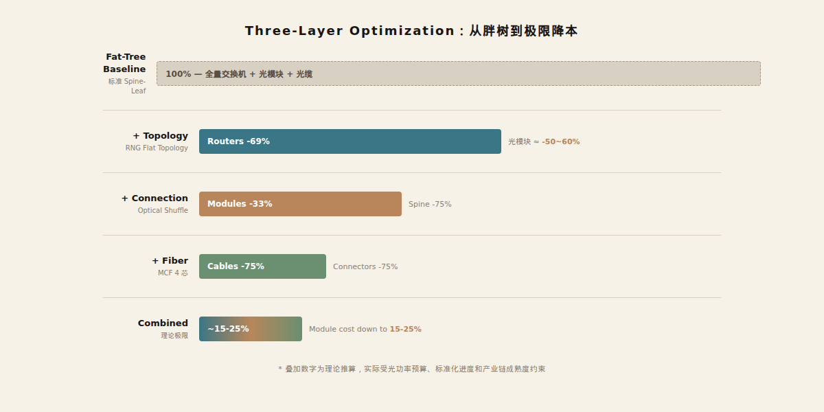
Theoretical limit of three-layer stacking:
| Optimization Layer | Approach | Effect |
|---|---|---|
| Topology | RNG flat topology | Routers -69%, transceivers -50~60% |
| Connection | Optical Shuffle | Transceivers -33% (of remainder) |
| Fiber | MCF 4-core | Cables -75%, connectors -75% |
| Combined estimate | All three stacked | Transceiver cost potentially down to 15–25% of fat-tree baseline |
This is theoretical — actual deployment faces optical power budgets, standardization timelines, and supply chain maturity constraints. But the direction is clear: topology + connection + fiber optimization, stacked, yields far more cost reduction than any single layer.
When Will Combined Deployment Happen?
Short term (2026–2027): Optical Shuffle deployed independently in 32K+ GPU clusters. Panduit is already pushing shuffle cable and panel standardization; AI cluster customers (large NVIDIA reference-design buyers) are natural first adopters.
Medium term (2027–2028): MCF begins deployment in Scale-Out layers of new AI data centers. Corning's product line is shipping; standardization gaps are closing through ITU-T processes. Key catalyst: fiber density bottleneck at 100K+ GPU clusters.
Long term (2028+): HCF deployed in specific Scale-Across scenarios (cross-building). Microsoft's precedent + gradually declining manufacturing costs open this market. Limited scale.
RNG + Shuffle + MCF combined deployment takes longer because it requires simultaneous topology and physical-layer changes. Most likely path: first optimize with Shuffle + MCF within fat-tree (no topology change), then consider flat-topology combination for GPU inference clusters after RNG-class architectures accumulate sufficient ops experience in non-GPU scenarios.
Conclusion
Castro's Optical Shuffle report appears to be a fiber cabling proposal. Underneath, it answers a bigger question: when AI clusters scale from 10K to 100K GPUs, where is the network cost bottleneck?
The answer isn't switching silicon — chip costs follow Moore's Law. It isn't topology — RNG has proven topology changes can eliminate 69% of routers. The answer is the physical layer — transceivers, fiber, and connectors. These components don't follow Moore's Law. Manufacturing process improvements are far slower than silicon scaling.
Optical Shuffle's 33% transceiver reduction isn't an isolated number. Combined with RNG's 69% router reduction and Corning MCF's 75% cable reduction, they form a complete cost-reduction path — from topology to connection to fiber, each layer with its own optimization space.
No one is doing combined deployment yet. But AWS's RNG has validated topology-layer optimization in non-GPU data centers, and Castro's Shuffle and Corning's MCF are validating connection-layer and fiber-layer optimization. When all three mature simultaneously, AI cluster network cost structure will change fundamentally — from "transceivers cost 3–5× what switches cost" to "network is no longer the primary cost constraint on GPU compute."
For China: the near-term highest-ROI move is following Optical Shuffle — no topology change, no routing change, just swap fiber jumpers and panels. Minimal ops disruption. MCF needs supply chain buildout. HCF needs more time. RNG-class flat topology is the most aggressive route with the largest payoff — but that's a topic for another article.
Disclaimer: This article is based on two public presentations by Panduit engineer Jose M. Castro at the IEEE 802.3 E4AI workshop (February 24, 2026): Optical Shuffle Architectures for Large AI Networks and Scaling AI Networks with Multicore and Hollow-Core Fiber, combined with public information from AFL Hyperscale, Corning OFC 2026 announcements, ITU-T MCF standardization proceedings, and Panduit's AI network cabling white paper. RNG references are from arXiv:2604.15261v3. Not investment advice. Data current as of June 7, 2026.
Related: A New Route for Data Center Networks: What RNG Opens Up