
From CED and CSA2 to Wide-EP, SWA bounded replay, DSpark, and asynchronous scheduling: a source-level teardown for AI infrastructure architects, product owners, and inference service operators.
Research scope: This article draws on official materials available as of October 23, 2026, and pins DeepInfer source code to commit
9bd9cf243fc53ef9afbf8f04d391d989117d6ab9. The method is documentation verification and static source analysis; we did not run our own GPU performance tests. Performance figures are separated into official disclosures, benchmark-script estimates, and this article's assumptions, and offline results are not treated as production promises.
The Conclusion First: Worth Serious Study; the Gains Come from Co-Design, and Production Still Needs the Rest of the System
DeepInfer's most important contribution is that it turns a set of DeepSeek engineering judgments into an implementation you can read, run, and verify. Once model serving enters the regime of long contexts, multi-turn agents, and large-scale MoE, the object worth optimizing is no longer a single matrix multiply, or tokens per second on a single card. It extends across the whole request lifecycle: how much computation is worth executing, how much state is worth keeping, which resources must genuinely wait for one another, and whether the system can convert those decisions into useful output that still meets latency constraints.
Its core advantage comes from co-design. The model reduces the KV that has to be generated and retained through CED and CSA2; the engine accepts an evaluable, approximate state reconstruction with SWA bounded replay, replacing expensive persistence and recomputation; Wide-EP redistributes Decode expert weights and batched compute across a large high-bandwidth interconnect domain; DSpark not only drafts tokens but exposes acceptance probabilities to the scheduler, so verification budget follows marginal return; asynchronous scheduling tucks the CPU work that used to sit on the critical path behind device execution. These mechanisms interlock, each creating preconditions for the next.
The other half of the conclusion matters just as much: what was released is the offline inference core that underpins a production system; DeepSeek's internal cloud service ships with considerably more. The repository already contains local KV allocation, state caching, batch scheduling, model execution, and many PD-disaggregation extension points. The distributed KV service, cross-instance routing and load balancing, and E/P/D service orchestration still have to be supplied by whoever deploys it. Reading "the internal production system is powered by DeepInfer" as "clone the repo and you get an equivalent production service" will be a very expensive lesson at launch time.[1][2]
The article first explains how the model changes computation and state, then moves through parallelism, speculation, and asynchronous execution, and finally puts benchmarks, economics, and productionization into a single acceptance framework. Readers who mainly care about technology selection can start with sections ten through thirteen, then return to the mechanism sections to check the preconditions behind each gain.
For teams already running large-scale DeepSeek business, with suitable scale-up interconnects and infrastructure engineering capacity, DeepInfer is a candidate worth putting through a validation pipeline—and a high-value sample for understanding the next generation of inference cost structure. For small-scale, multi-model teams that prize out-of-the-box operation, it is first an architecture reference and a target for targeted experiments, not necessarily the unified serving foundation to adopt right away. The final choice should be decided by service quality under real request traces, effective throughput, capacity risk, and total cost—not by a Pareto chart published on launch day.
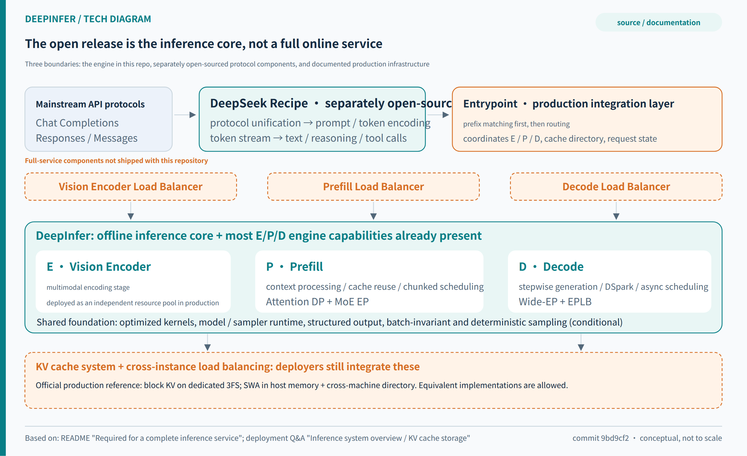
How to read Figure 1: the open core solves "execute one inference well"; a complete service must also solve "get the request and its state to the right place, and keep working through failures". The outer components mark the production responsibility boundary; that does not mean the repository entirely lacks the underlying capabilities.
One: From Chat Server to Token Factory—Why the Bottleneck Moved
Early LLM deployment was typically about fitting the model into video memory, making single-request responses fast, and raising utilization with batching. Today an agent may repeatedly read tool results, retrieve documents, and edit code, carrying an ever-growing history every turn. Input length, output length, inter-turn gaps, and prefix reuse rates now shape cost as much as parameter count. The same "million tokens" may be a mass of first-turn long inputs with no reuse, history context that hits cache over and over, or long outputs that continuously occupy Decode resources. Reporting a single blended token price hides the real resource consumption.
Prefill and Decode are not the same kind of work, either. Prefill processes one known input segment at a time and can usually form large matrix computations; Decode must advance along autoregressive dependencies, with each step contributing limited useful work per request, making it more sensitive to weight movement, KV reads, communication, and scheduling gaps. Long context further raises attention state and access costs. Multimodal workloads add a separate visual-encoding stage whose cost depends on image size, tiling, and patch count.
So "keeping the GPUs busy" says little by itself. GPUs can be busy recomputing prefixes that could have been reused, verifying drafts that will mostly be rejected, waiting for other ranks, or producing output the client already cancelled and will never receive. What a token factory must raise is how much useful result each unit of total resource delivers at a given quality and service level.
DeepSeek's deployment Q&A is quite concrete about the target: support multiple accelerator vendors; organize Prefill on ordinary eight-GPU machines and Decode on 64–128-GPU-class supernodes; keep KV reusable for more than 72 hours. These are constraints imposed jointly by procurement, networking, storage, and business shape—not abstract algorithmic metrics.[2] Understanding this set of constraints is worth more than memorizing any optimization buzzword. A solution that fits large-scale agent traffic may not pay off the same way at low concurrency, low reuse, and small models.
Seen from this angle, DeepInfer demonstrates how model structure makes scheduling, caching, and hardware deployment more favorable—the answer to cost does not lie entirely in the scheduler. The model decides which states must exist; the system decides where those states live, when they are produced, how they migrate, and how long they remain worth keeping.
Two: Get the Release Boundary Right—Runtime, Service Plane, and Internal System Are Three Different Layers
The README states plainly that this release provides offline inference, lists DeepSeek-V4.1-Flash as the currently supported model, and names two hardware targets: NVIDIA SM100 and Huawei Ascend 950. Dependencies include Linux, GCC 13+, Python 3.12; the NVIDIA path requires CUDA 13, the Ascend path CANN 9.2. This is the range officially supported today; other model and hardware combinations should not be taken as verified on this basis.[1]
The open runtime is far from thin. The outer LLM interface handles inputs, sampling parameters, and request lifecycle; LLMEngine stitches batch scheduling, state management, and device execution together; the C++ side carries sequences, block management, scheduling, and input metadata; the Python side organizes models, graph execution, operator backends, and platform adaptation. The README also documents structured output, deterministic sampling, batch-invariant inference, DSpark, and bounded replay. This is not a showcase project with a handful of kernels.
A complete online service, however, involves another class of problems: request authentication and quotaing, protocol translation, queueing and cancellation, cross-instance routing, retry on failure, session migration, distributed cache lookup and transfer, autoscaling, metering, and observability. The README lists a KV cache system, VE/Prefill/Decode disaggregation, and load balancing across Prefill and Decode data-parallel replicas as components a full service still needs. "Missing KV system" here refers to the distributed service layer—not the absence of local KV caching.[1]
The distinction is directly verifiable in source. deepinfer/worker/cache_engine.py implements KVCacheManager, GPUCacheInterface, StateBlock, and GPU cache allocation; csrc/engine/block_manager.hpp manages block resources; LLMEngine retains extension hooks such as init_pd_split, post_schedule, do_save_kvcache, and send_processed_prompts. They show the engine has thought about where a production system plugs in; they do not turn the not-yet-integrated storage, transfer, and routing into delivered services.[3][4]
One more easily confused boundary: the README capability table includes balanced CP, while the official Q&A says the current internal deployment does not use TP or CP. There is no contradiction. The former is the implementation support surface; the latter is a production choice under a particular model, hardware, and workload. An architecture assessment should record "can run", "validated", and "officially adopted today" as three separate states rather than collapsing them into one checkbox.
Three: Model–Engine Co-design—First Reduce the Work That Must Be Done, Then Accelerate What Remains
CED treats the Prefill and Decode computation graphs differently
The DeepSeek-V4.1-Flash technical report gives a 552B backbone, with roughly 8B parameters activated per token in Prefill and about 16B in Decode. The asymmetry comes from Causal Encoder-Decoder, CED for short—not from running the same network at two precisions.[5]
Do not map "encoder" and "decoder" here onto the classical machine-translation mental model: the encoder remains causal in its computation, and it is not the "E" of the system-level E/P/D split (that E is the vision encoder). CED is a topology inside the model; Prefill/Decode disaggregation is a deployment topology of the service. They compose, but they are different things. The front half of CED is a stack of causal encoder layers; in the back half, the global KV is no longer produced by every layer processing the full prefix, but is projected from the last encoder layer's hidden states. For a complete history, the global memory the Decoder part needs can be established through this shorter path. Prefill therefore does not have to run full token-by-token computation across all layers.
Why does Decode still need the fuller path? Because producing the current token's hidden state and output still requires the corresponding deep processing, and each layer's local sliding-window state keeps its own layer-wise dependency. What CED removes is the duplicated work of building state from historical input; it does not make the back half of the model disappear from generation. "Prefill skips computing much of the history; Decode keeps the ability to generate" is a more accurate reading than "the model is cut in half".
For input-heavy, tool-calling agents this structure pays off directly. After a tool call, the system must absorb the new input while the prior history may still be long. If the model makes building historical state cheaper, both cache-hit and cache-miss scenarios become easier to control for TTFT. The gain still scales with input size: when inputs are already short, or the request's cost is dominated by a long output, Prefill optimization cannot cut end-to-end cost by the same proportion.
CSA2 splits the duplicated storage and duplicated indexing of global memory
Reducing Prefill compute alone is not enough. Long-context serving is constrained by KV capacity, load bandwidth, and storage cost simultaneously. CSA2—Compressed Sparse Attention 2—splits cross-layer sharing into three modes: Full, Reindex, and Reuse. A Full layer generates global KV and indexes it; a Reindex layer shares the global KV that already exists but re-selects relevant entries with its own queries; a Reuse layer reuses even the selected Top-K indices. Meanwhile, every layer keeps its own global Q and local SWA KV.[5]
The key admission in this design: not every layer needs to re-create a copy of historical memory, and not every layer needs to re-decide which history to read. Sharing "store memory" and "select memory" separately can allocate computation more flexibly than one-size-fits-all reuse. It also means the attention backend is no longer a homogeneous layer-by-layer structure. An implementer must know whether a layer is a producer, a re-indexer, or a consumer, or the cache layout, lifetimes, and operator calls can all go wrong.
To make the three modes' boundaries concrete, a compact responsibility table:
| CSA2 mode | Global KV / indexer K | Top-K selection | What the layer still computes itself |
|---|---|---|---|
| Full | newly generated | newly selected in this layer | main query, local SWA, attention output |
| Reindex | reuses existing state | re-selected in this layer | main query, local SWA, attention output |
| Reuse | reuses existing state | reuses existing selection | main query, local SWA, attention output |
V4.1 uses pure CSA2, not the V4 CSA/HCA mixture. Of the 40 backbone layers, the first 20 are causal encoder layers and the last 20 are decoder layers; under the reported configuration there are only four main global-KV sources, not one per layer. Reuse is not copying the previous layer's output, either: the current layer still processes the selected memory with its own queries. That preserves cross-layer expressive variation while cutting duplicated state.[5][11]
Work out the 890 B/token before claiming what was saved
Each main-KV entry holds 512 four-bit values: 256 B of data, plus one scale byte per 16 values—288 B in total. Each indexer-K entry holds 128 four-bit values: 64 B of data plus one scale byte per 32 values—68 B in total. Three encoder global caches are produced per two raw tokens, and one decoder global cache per token, so the ideal global KV footprint checks out as:
(3/2 + 1) × (288 + 68) = 890 B per raw token.
That number bundles three optimizations at once: sharing decides how many copies, sequence compression decides how many entries per copy, and numeric format decides how many bytes per entry. For 1,048,576 tokens, the ideal capacity of these global-KV entries alone is 890 MiB; that is not the full memory footprint, and it certainly does not imply the model runs on a single card. Weights, Engram, SWA, draft state, scratch workspace, page metadata, communication buffers, and graph-execution memory all sit outside this small ledger.[5][23]
Storage precision and compute precision must also be kept apart, and "uses FP4" must not be read as "every tensor is four bits": main-KV FP4 mainly saves state; values are dequantized before attention computation, so the whole attention path is not doing FP4 matrix multiplication. The Q&A describes separate quantization formats for main KV, indexer KV, and routed-expert weights; SWA uses the MXFP8 format, where each cached position in each layer takes 528 B — 512 B of data plus 16 B of scale factors — and the total also depends on how many layers are kept and the window length. System gain depends on the total size of data, scales, alignment, indices, and metadata — and on their read/write patterns — not on ideal bit counts alone; dividing a chip's advertised FP4 peak throughput by model FLOPs will not predict this mixed-precision, sparse, memory-bound path.[2]
After sparse attention, finding the relevant history itself costs something
The global attention branch reads at most the 512 selected entries, plus an independent local SWA window; that does not mean locating those 512 entries is free. If every indexing layer still scanned the full history, indexing overhead would become the bottleneck again at long context. V4.1 avoids repeated indexing with Reuse layers, and has the decoder's first Full layer form a candidate pool while scanning history: at most 2,048 eight-position blocks, yielding up to 16,384 candidate positions; subsequent Reindex layers then pick their own Top-512 from the pool.[5]
16,384 is the retrieval range; 512 is the final main-attention selection—the two must not be conflated. The candidate pool is also not a permanent summary of the whole session; it is shared information produced along with the query. Hierarchical indexing bounds later retrieval to a fixed-size set, but the initial global scan still grows with history. The accurate conclusion is "the growth of long-context dominant cost is suppressed", not "Decode becomes context-independent O(1)". It also introduces a quality boundary: important history missed by the early candidate set may be unrecoverable in later layers, which deserves dedicated evaluation on distant-evidence, rare-reference, and multi-step tool tasks.
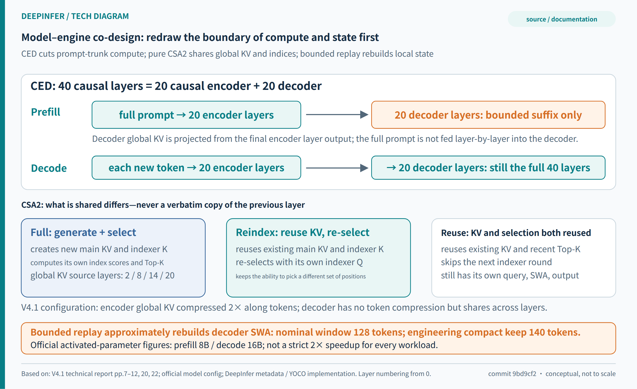
How to read Figure 2: CED inside the model is not the service-level P/D split; cross-layer KV reuse, index reuse, and bounded decoder replay each remove a different kind of work. The 890 B/token figure describes global KV only, not full device memory.
The official report states that at equal sequence length, V4.1-Flash runs at about one quarter the runtime KV of DeepSeek-V4-Flash, and about one eighth for persisted KV. Those are relative figures produced jointly by model architecture, precision, and caching strategy—not a universal compression ratio DeepInfer provides for arbitrary models.[5] Likewise, Decode FLOPs growing slowly with context does not mean end-to-end latency is flat in context: indexing, memory access, cache loading, and queueing can still shift.
Beyond attention and MoE: conditional memory and residual paths have system bills too
Engram and Single-Pass mHC are two more pieces of the co-design. Engram addresses a conditional memory table by n-gram hash of the input tokens, then projects and gates the retrieved content into the hidden state. The open runtime shards the table across a dedicated parallel group and handles cross-rank lookup; its addressing is determined by the input, which creates room for prefetch–compute overlap. But the capacity and communication of large-scale conditional memory do not vanish from the deployment budget, and "activated parameters per token" alone cannot measure them.[5][24]
Single-Pass mHC and Mega-mHC are a reminder that activation traffic in residual and mixing paths deserves optimization too. This is not merely fusing a few kernels of the original graph: Single-Pass mHC first changes the dependency of the input-mixing coefficients, using the previous block's coefficients to remove the original wait; Mega-mHC then fuses residual update, coefficient computation, input mixing, and pre-normalization. The official report states the fused Mega-mHC halves activation memory traffic on this path versus the original four-kernel implementation; that is not "total model memory, total runtime, or all memory access halved".[5] Once matrix computation and attention are highly optimized, these formerly unremarkable repeated read-writes, normalizations, and launch costs become the new bottleneck. Full performance requires walking the whole execution trace to find the gaps; staring at the largest operator is not enough.
Co-design also means transferability has limits
These gains are attractive precisely because the model created the conditions at training and structure level. Wiring DeepInfer onto an ordinary Transformer not designed the same way will not automatically yield half-priced Prefill or the same cache compression. The quality impact of SWA bounded replay is likewise decided jointly by model structure, training adaptation, and task distribution—not a mathematical identity that holds for every model.
So there are two different reasons to study DeepInfer. One is deploying the current models: reproduce as much of the validated combination as possible. The other is absorbing the architectural ideas for your own models or serving stack: that requires re-validating accuracy, scheduling, and cost, not just porting config names. It is also exactly why model teams and systems teams need to collaborate early—once a model ships, many cost boundaries are already written into its computation graph.
Four: SWA Bounded Replay—A Quality-Bounded "Store Less, Compute Less"
Why local windows can still create an expensive recovery problem
Sliding-window attention looks cheap: each position reads only the last W tokens, and state size does not grow linearly with total context. But once layers stack up, a deep layer's recent-window hidden states still depend on earlier layers and farther positions. Exact reconstruction of deep SWA state would unfold the recovery range across layers; recomputing one window is not automatically enough.
In V4.1's decoder setting, the Q&A contrasts the most recent 2,560 tokens needed for exact recovery with the roughly 128 most recent tokens used by bounded replay. The latter allows SWA access only inside the replayed segment: replaying from position s, position i reads local keys only from max(s, i−127) through i. It deliberately truncates local dependencies outside the replay segment, so what it reconstructs is approximate state.[2]
The value of this move goes beyond "somewhat faster". If an SWA cache miss must trigger an expensive long-segment recovery, the system has to spend a large storage budget guaranteeing state never drops; once a miss costs only a bounded, predictable short replay, SWA can live in a cheaper short-term memory tier and be reclaimed without anxiety after expiry—the economic boundary between storage and computation has been rewritten.
Encoder and decoder replay solve different problems
Encoder bounded replay addresses "global block KV hit, but SWA state not found". The system reuses the hit global KV, additionally replays a short tail of the pre-hit prefix to rebuild local SWA state, then continues with the uncached input suffix. The replay segment restores SWA; it must not recompute or overwrite the reused global block KV. This saves compute and protects the hit KV—but the newly generated global KV and SWA of the uncached suffix are still affected by the approximate state, and different hit boundaries are not mathematically equivalent.[2] The direct discussion is on page 20 of the technical report.
Decoder bounded replay is what lets CED actually cash in its Prefill savings. The decoder global KV for the full history can already be projected from the encoder output; what remains is the local SWA state of each decoder layer. So only the tail window passes through the decoder, producing the local state subsequent Decode needs. This reconstructed state serves the current generation; it does not enter the persistent prefix cache.
Bounded replay is thus both the fallback for cache misses and a component of the model's computational-graph optimization. The former lets long-term cache skip storing one expensive kind of state; the latter lets Prefill skip executing long decoder segments. The two are related, but should not be conflated into a single "cache compression switch".
Why 128, 134, and 140 appear at the same time
The official mechanism explanation uses a 128-token window; the Q&A's SWA state slots and prefix-hit bound involve 128 plus 6 positions; the README's recommended decoder keep length is DEEPINFER_YOCO_PREFILL_KEEP_TOKENS=140. These numbers hold different responsibilities: window width describes attention dependency; the extra positions serve speculative rollback and ring-buffer state boundaries; the kept suffix is an implementation safety configuration.[1][2]
Do not mechanically set production config to 128 because a principle diagram says 128. The keep length must at least cover the window plus maximum rollback demand, and must match draft length and the state implementation. After changing these parameters, check the storage points around the 128 boundary, rollback after draft rejection, the last chunk of chunked Prefill, the first Decode step after recovery, and state reclamation on request cancellation.
The repository also provides equivalence verification between mask and compact implementations. Masking shields unneeded parts in the original layout; compact squeezes the actually executed data together to remove useless work. examples/yoco/yoco_equiv.py compares metadata, visible keys, and storage slots at L1; at L2 it compares logprobs and Top-K on a fixed teacher-forcing trajectory, and can check draft confidence.[6] What this verifies is that the two truncation implementations agree—not that bounded replay is mathematically equivalent to full-history computation. The latter is approximate by design and requires separate task-quality evaluation.
Five: Cache Becomes Its Own Infrastructure—Why One HBM→DRAM→SSD Arrow Is Not Enough
A generic multi-tier cache diagram draws HBM, host memory, and SSD as one hot-to-cold chain. DeepSeek's published deployment design is more pointed: the block KV and states being computed live in device memory; SWA's short-term reusable state lives in the production machine's host memory; long-term paged block KV lives on a dedicated 3FS storage cluster. Different content has different lifetimes and does not have to pass through identical tiers.[2]
Global KV is worth persisting because it may be reused by many requests long after it was written. SWA is more like local working state while a session advances: once the user moves to the next turn or the session ends, the old state's value decays quickly. The official technical report accordingly places SWA in a short-term host-memory pool, keeps global KV in long-term storage, and relies on bounded replay to handle SWA misses. What is being optimized is the state's future reuse value, not total cache volume.[5]
Separate storage also pays off at the routing layer. If a prefix exists on only a few Prefill nodes, the scheduler must choose between "go where the cache is" and "go where capacity is free"; shared storage lets any Prefill node read a hit prefix, easing the conflict between cache affinity and load balancing. It also decouples compute-node failure from long-term cache loss, so storage scaling no longer has to track compute resources one-for-one.[2]
The costs are equally clear: a hit that once completed in local memory may now involve directory lookup, network read, host shared memory, and HBM import, so the system needs good enough tail latency and overlap capability. The Q&A describes matching, reading, and swap-in separately: matching queries metadata only, but hit length influences routing and cannot be fully hidden; KV pull proceeds asynchronously in a separate process; host-to-device import proceeds layer by layer with the goal of overlapping compute. The internal NVIDIA path also uses GDR for fine-grained cache-block transfer through RDMA NICs, avoiding SM occupation.[2]
A cache system with a beautiful hit rate but slow recovery can worsen first-token latency. A deployer must measure hit length, hit bytes, metadata-query p99, first-layer-ready time, all-state-ready time, I/O–compute overlap ratio, and the cost of recomputation after a failed pull. A single "share of requests with cache hits" cannot answer how much compute was actually saved.
The internal scale disclosed in the Q&A is large: roughly 100 PiB of SSD capacity, about 14.4 TB of logical cache per GPU, and TTLs of three days for agent traffic and seven days for chatbot. The recommended storage node uses twenty 30.73 TB SSDs with at least 40 GB/s read and 5 GB/s write.[2] These are engineering parameters of a reference deployment, not install thresholds for DeepInfer. TTL, physical redundancy, and cache capacity should be derived from your own reuse curves; copying the capacity only copies the bill, not necessarily the hit rate.
Nor should these caching capabilities be read as "Decode reads KV from SSD token by token". The Q&A states explicitly that internal Decode does not enable KV offload: state for in-flight requests stays on device; the KV Decode produces is written to persistent storage for future requests to reuse. Long-term storage and the current generation's critical path are two different uses.
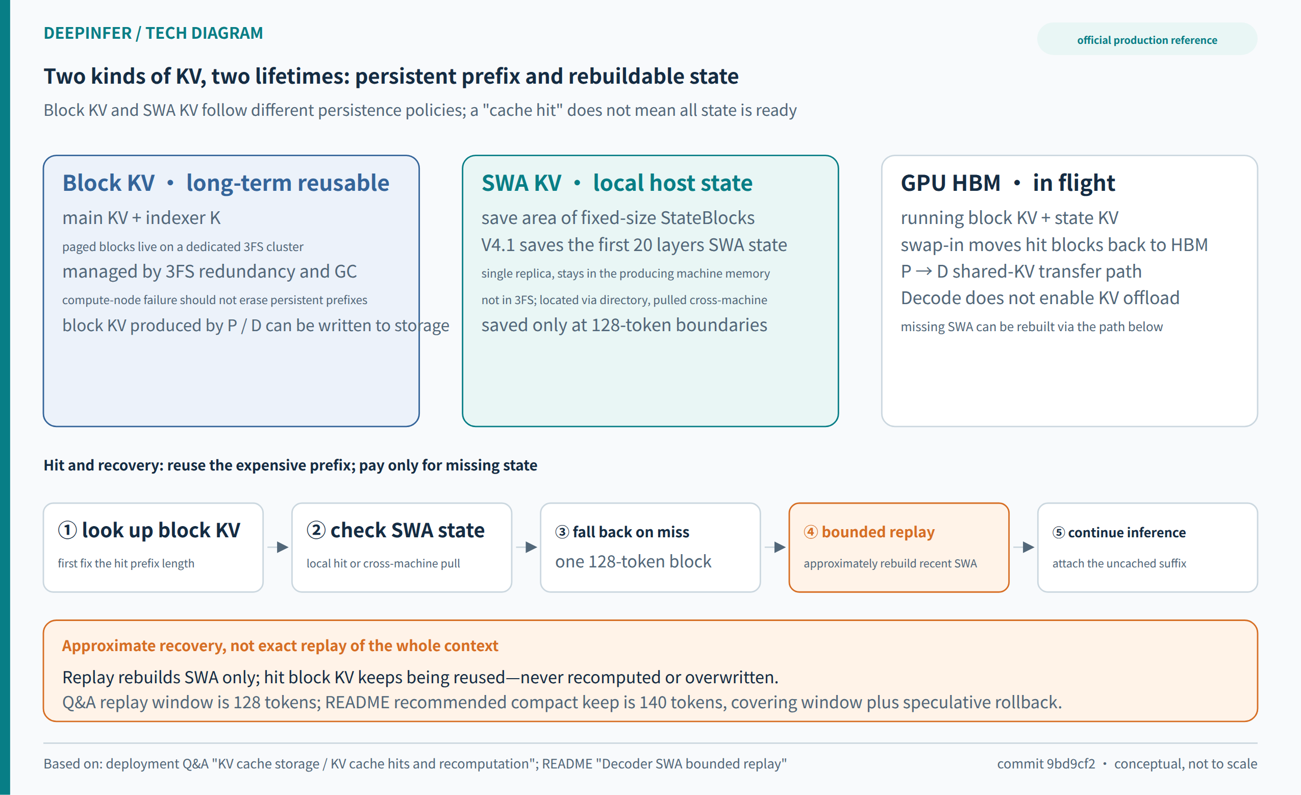
How to read Figure 3: long-term block KV and short-term SWA are managed separately; a missing SWA can be recovered by replay, and a long-term global-KV hit does not have to be discarded because of it. The asynchronous reads and layer-wise loading describe the official internal design; the open repository still expects external storage services to be attached.
Six: Attention DP, Wide-EP, and EPLB—Rearranging the Waiting
One request table, two parallelism views
For a MoE model, attention and expert computation do not necessarily want the same parallelism. DeepSeek's deployment runs attention data-parallel by request: each rank serves its own requests and holds the corresponding KV; at the MoE stage, tokens are dispatched by routing outcome to the devices owning each expert. The same set of devices is thus both a DP replica group for attention and an EP member group for MoE.[2]
Why give Decode a very wide EP? Each decoding request contributes only a few tokens per step; an expert seeing a tiny batch cannot fill the device with matrix work and must still stream large amounts of expert weights. Holding per-rank concurrency roughly constant while total traffic grows with the domain, packing more requests into one expert-parallel domain raises the effective batch per expert and spreads expert weights across more devices, easing per-card weight movement per step. If total traffic is fixed and small, a wider domain creates no useful work out of thin air and may only add communication and idleness.
The preconditions go beyond "having 64 cards". Tokens must dispatch across ranks and combine back to their owning requests; expert execution waits for the slowest member of the synchronized domain. With high network latency, insufficient effective bandwidth, or a few very hot experts, what gets amplified may be communication and waiting. The official Decode benchmarks run within one scale-up domain; that physical boundary should be read together with the EP64 numbers, not extrapolated to an ordinary Ethernet-connected 64-card cluster.[1]
Prefill chooses differently. A large input block already provides a large compute batch, and widening EP further may not be worth the extra communication. The Q&A therefore suggests the smallest EP/DP HBM allows for Prefill (examples EP2–8) and the widest EP/DP the hardware supports for Decode (examples EP64–128). The two stages are seeking different compute–communication balance points; there is no conflict between them.[2]
EPLB balances the slowest device at each step
Distributing 384 experts evenly across GPUs does not distribute load evenly. Model routing shifts with task, language, context, and generation phase. Some experts stay hot; others spike only at specific moments. In synchronized execution, idle average GPUs cannot compensate for one very busy rank, because the next step still waits on the slowest.
EPLB separates the model-semantic logical expert from the physical expert replicas in deployment. Hot experts can have multiple physical replicas placed into fixed slots on each GPU. What makes the open policy.py interesting is that it optimizes placement using per-step historical load, targeting something close to "the sum of the slowest rank's load per step"—not merely equalizing token counts over the whole statistical window. Two experts that run hot at different times may share a card reasonably; two that always run hot together can create spikes despite identical average statistics.[7]
The Q&A gives starting parameters by phase: Prefill starts at four redundant experts per GPU, a 100-step statistics window, and redistribution every 1,000 steps; Decode starts at one redundant expert per GPU, a 1,000-step window, and redistribution every 10,000 steps. "Starting" matters: final physical expert counts are further constrained by divisibility and capacity. The numbers reflect different timescales, hot-spot dynamics, and migration costs between Prefill and Decode—not a recommendation to copy parameters across all traffic.[2]
EPLB has costs too: redundant experts occupy HBM, weight redistribution consumes communication and execution time, overly frequent adjustment chases noise, and overly slow adjustment misses load shifts. Production monitoring should record not just average expert token counts but the slowest/average rank ratio, redistribution events, weight-migration time, and tail latency before and after adjustments. For multi-tenant businesses with fast task switching, also check whether mixed tasks make the statistics window unrepresentative.
Mega-MoE's fusion depends on topology and layout contracts
Mega-MoE fuses communication and expert-compute paths more deeply, cutting intermediate tensor movement, kernel launches, and inter-stage gaps. The open code does not unconditionally take the fused path in every environment: enabling conditions involve whether the EP group sits within a physical scale-up domain and the supported precision combinations; other cases retain the explicit dispatch, grouped GEMM, combine path.[8]
This is a point easy to miss when reading inference-framework code. High performance is usually not one smarter function: the upstream gate writes indices and weights directly into an agreed communication buffer, inputs arrive in a predetermined format, and the downstream kernel skips re-shaping. Change the data layout at any layer and the fusion gain can evaporate. What an architect manages is a set of cross-module contracts; swapping a single operator does not buy this gain.
Wide-EP also enlarges the failure domain. The Q&A notes that a single GPU failure inside a large EP instance makes the whole communication instance unavailable; the internal system relies on redundant capacity and request-level rerouting, and re-determines EP size from healthy GPUs on restart.[2] A wider EP can therefore raise steady-state efficiency and simultaneously raise the number of requests affected when a failure occurs. Procurement must evaluate effective throughput together with failure recovery.
The official "64 Prefill plus 64 Decode as the minimum efficient deployment unit" should be read against its recommended EP64 and actual P:D of roughly 1:1. The same Q&A says 1P+1D is deployable. The former is a reference configuration for particular business and efficiency targets—not the software's minimum hardware requirement, and not a conclusion that every enterprise must buy 128 cards to start experimenting.
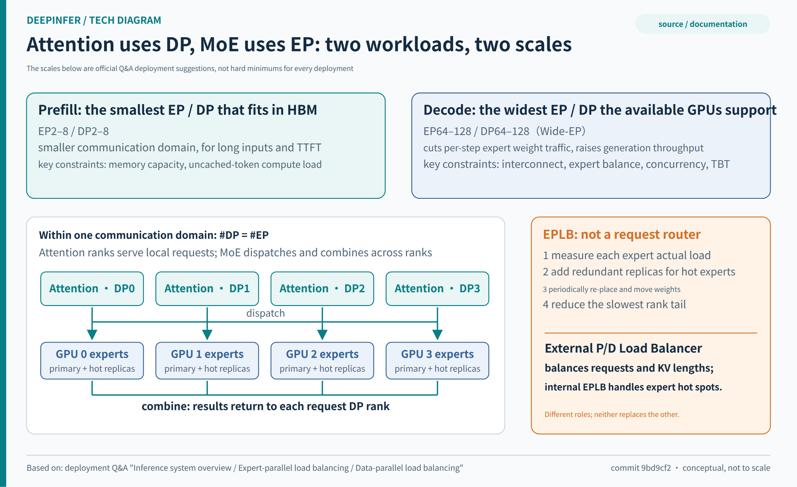
How to read Figure 4: attention preserves request locality while MoE exchanges tokens inside the high-bandwidth domain; EPLB uses physical replicas and placement to reduce slow-rank drag. A wider EP must be judged together with communication conditions, load balance, and failure domain.
Seven: DSpark—The Verification Budget Is Scarcer Than Drafts
Why generating more drafts can make the system slower
Speculative decoding uses a cheaper draft path to propose several candidate tokens, then verifies them in one batched pass of the target model, hoping one heavier forward advances several positions. Its payoff depends on the relation between draft cost, acceptance length, and verification cost. A request being able to propose five tokens does not make verifying all five optimal: later candidates easily lose value when an earlier one is rejected, yet verifying them still consumes compute.
DSpark adds two kinds of information. First, the draft is semi-autoregressive: a three-layer draft Transformer produces base information for five positions in parallel, and a lightweight Markov head models dependencies among candidates. Second, a Confidence Head estimates each position's conditional acceptance probability, letting the scheduler predict the yield of converting a draft segment into output.[5][9]
The probability is not "high confidence, so skip target-model verification"—Confidence only decides which prefixes deserve the verification budget; final acceptance is still decided by the speculative-sampling check. Nor may intermediate positions be skipped arbitrarily: the request advances along the prefix; for later candidates to pay off, earlier candidates must survive first.
From fixed length to marginal-gain budgeting
If p(i,j) is the conditional acceptance probability of candidate j for request i, then when verifying up to position k, the expected increment from drafting can be written intuitively as a sum of prefix-survival probabilities: p(i,1), plus p(i,1)×p(i,2), and so on. Add the target path's baseline progress. The objective is the batch's expected effective output per step time; maximizing total candidates, maximizing average acceptance, or pushing one request furthest are all proxy metrics.
These objectives can conflict. Picking only the trivially accepted first draft yields a beautiful acceptance rate but may leave hardware underused; fixing five candidates for every request fills the batch but may waste compute on low-yield suffixes; chasing the longest advance for one request can damage other requests' interactivity. DSpark combines confidence with hardware throughput curves to find a suitable total verification budget for the current load, then allocates it across requests.
The open code makes this concrete. csrc/engine/mtp_varlen.hpp uses a Decode performance curve captured at startup, adds runtime forward and sampler time estimates, and compares expected gain per time across graph sizes; the estimate does not treat one offline profile as permanently correct—runtime refines it with actual execution feedback, because context length and request mix change runtimes.[9]
It shares a timing constraint with asynchronous scheduling that must be preserved
Under asynchronous execution, when the CPU plans the next schedule, the latest round of Confidence may not have returned. Forcing a sync to obtain it would forfeit the scheduling overlap. DeepInfer's approach: the CPU first decides the total budget, then the GPU refines per-request verification lengths with fresher information. The source further distinguishes confidence from different rounds for batch budgeting versus request lengths, preventing information about future positions from improperly influencing earlier candidates' verification choices.[9]
This explains why DSpark cannot be understood in isolation as "one more prediction head". It connects the draft model, sampling semantics, a runtime performance model, graph sizes, request mapping, and CPU/GPU timing. When modifying the scheduler, keeping only aggregate throughput while dropping these constraints can introduce selection bias or state errors while appearing faster.
The official Q&A's dynamic-versus-fixed-five comparison is restrained: at roughly 60 concurrent requests per rank, estimated throughput rises from 13,730 to 14,466 tokens/s/rank, about 5.4%; at 16 concurrency it is −1.5%, and at 96 concurrency +11.0%.[2] Saving wasted verification pays off more at higher load, and a dynamic policy does not win at every operating point. "About 4%–7% at the production point" must not be rewritten as a guaranteed speedup in any environment, let alone multiplied with improvement ratios from another paper, model, or draft version.
Acceptance rates also drift by task. Code, natural language, structured JSON, long reasoning, and multilingual text need not draft equally well. At launch, watch whether predicted and actual accepted lengths stay calibrated per task bucket, and record budget-algorithm error, sampling time, draft time, and tail latency together. A stale throughput curve and an overconfident predictor can both make the optimizer stably choose the wrong operating point.
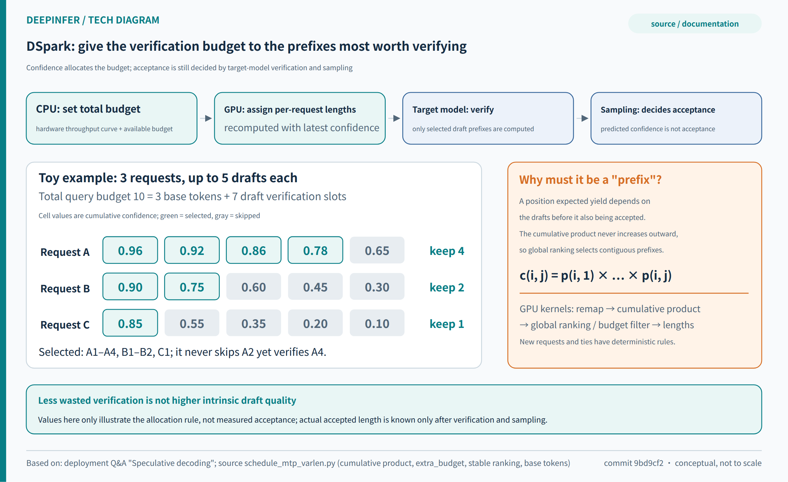
How to read Figure 5: budget goes first to candidate prefixes with higher expected yield; gray suffixes can go unverified; "predicted worth verifying" (green) does not mean accepted by the target model. The objective is effective system output per time, not draft length.
Eight: Asynchronous Scheduling—Hiding the CPU Gaps Also Surfaces Lifecycle Problems
A synchronous inference loop executes schedule, forward, sample, sync, post-process, then starts the next step. While the device finishes sampling and the CPU reads results and prepares the next batch, the GPU may have nothing to run. As kernels get faster, the formerly invisible Python and C++ bookkeeping and object management become a fixed per-step tax.
DeepInfer's "zero-overhead batch scheduler" should be read as hiding this tax as much as possible—not as the CPU work vanishing. The open Worker logic launches the current forward, processes the previous round's results while the device runs, then launches the current sampling; CPU and GPU advance as a pipeline. Lagging sequence lengths and request mappings are repaired by a device-side metadata-correction path, avoiding a full sync every step just to obtain the latest results.[10]
Why does this overlap matter? Suppose a GPU step takes time G and CPU bookkeeping takes C; the synchronized critical path is roughly G+C, while proper overlap approaches max(G,C) in the ideal case—residual unhidden dependencies and launch costs remain. It matters most for short-step Decode, where fixed CPU overhead is a larger share of each step. Conversely, if schema compilation, network callbacks, memory copies, or cross-rank coordination slow the CPU so that C exceeds the hideable window, device gaps come back.
The price is that the temporal "now" gets complicated. When the CPU believes a request has finished, the device may still be reading the previous step's metadata; a state block removed from the logical queue cannot necessarily be reused immediately; the element at the same position in a new batch is not necessarily the same request as in the old one. DeferredRelease, block reference counts, pin/unpin, and event synchronization in the source exist precisely to maintain these invariants.[3][10]
This point decides whether production integration is safe. LLMEngine.step() states explicitly that returned RequestOutput objects come from an object pool and are recycled on the next step; keeping them across steps requires clone. An HTTP/SSE service that pushes internal objects directly into an async send queue may have the engine reuse memory before a slow client has finished reading. The correct pattern is to copy stable output events at the boundary and let an independent network layer send them, with a bounded send queue. Throughput optimization must not assume clients are always fast enough.
Request cancellation, timeout, and rolling shutdown must also cover in-flight state. The source provides flush_inflight_reqs to settle unaccounted outputs in the ZOS pipeline; this belongs in the engine-drain procedure, not merely in stopping calls to step. Tests should cancel requests between Prefill, verification, sampling, and output delivery, and verify no double billing, duplicated output, premature release, or leaked resources.
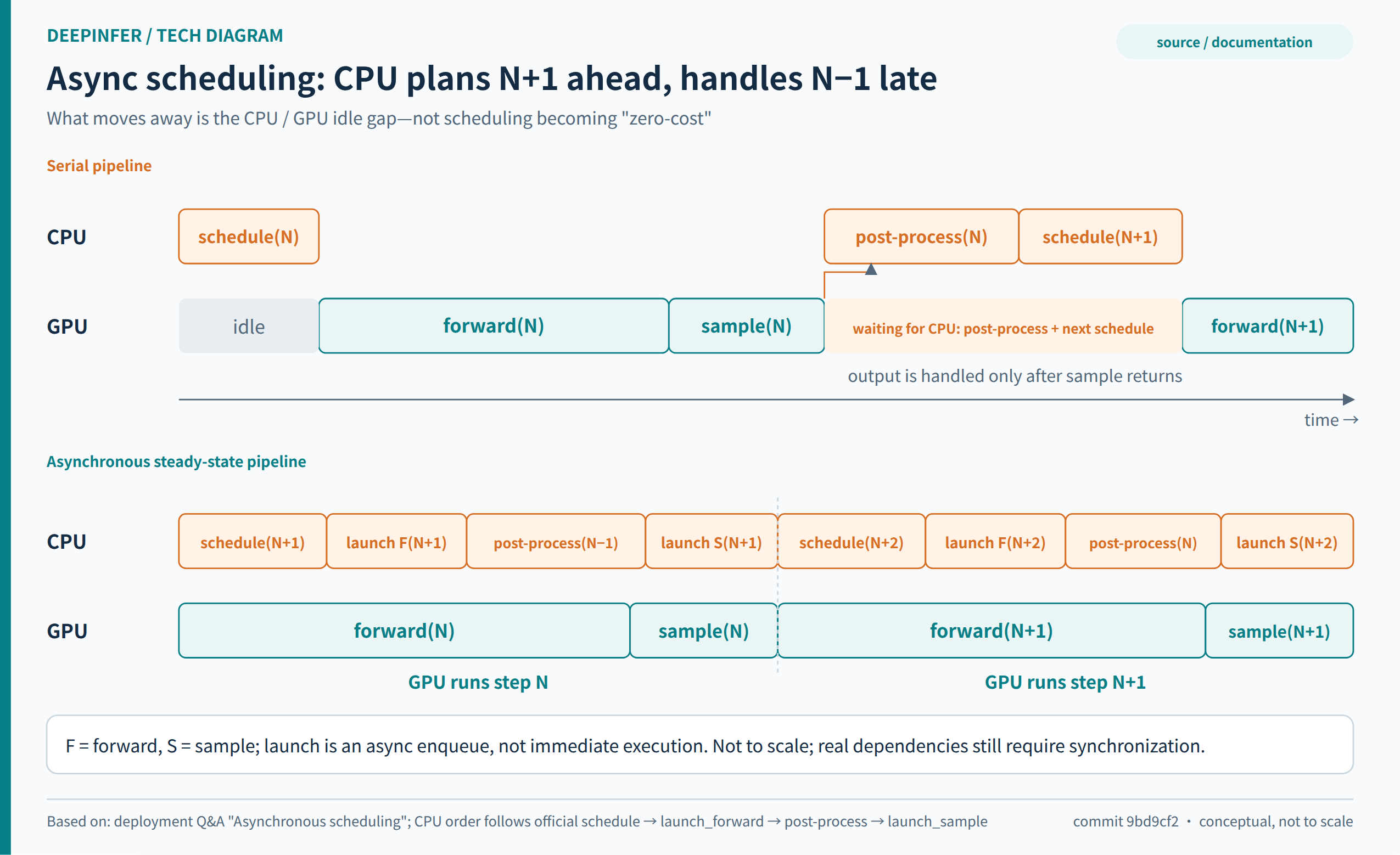
How to read Figure 6: what overlaps is the parallelizable CPU scheduling and prior-result processing with device execution; the dependencies do not disappear—they are moved off the critical path through stricter state and buffer lifetime management.
Nine: Reading the Implementation—Walk One Request Through, Don't Get Lost in the Operator Directory
The most effective way into this repository is to walk the request path first, then descend into hot spots. examples/offline_inference.py shows startup, model configuration, and output checking; LLM.generate in deepinfer/entrypoints/llm.py enqueues requests, loops step, and drains in-flight results at the end. That is a comprehensible offline entry point—not an online continuous-batching service you get by wrapping the whole function in an HTTP handler.[3]
The second stop is deepinfer/engine/llm_engine.py: worker initialization, cache initialization, request admission, post-schedule processing, and extension hooks. Following self.scheduler.schedule() inside step leads to csrc/engine/scheduler.hpp, where you can see how sequences batch, how state is allocated, and how chunked Prefill advances. Then csrc/engine/input_metadata explains how a logical request becomes device-consumable indices, lengths, and cache-load plans.[4]
The third stop is deepinfer/worker/worker.py and model_runner.py, connecting async timing, graph execution, model forward, sampling, and performance feedback. Only afterwards does v4_modules—shared-layer topology, YOCO, attention, and MoE—make sense, including why a consumer layer does not do all of a producer layer's work. The shared-relationship checks in cross_layer.py exist precisely to keep reuse logic from reading state that has not been written yet.[11]
The fourth stop is specific kernels. FlashMLA, DeepGEMM, DeepEP, TileKernels, DeepSelect, and the TileLang operators in the repository each carry different duties: attention, matrix computation, expert communication, fine-grained fusion, index selection, and runtime metadata handling. examples/benchmark.py can generate traces; find where time actually goes in a real trace before deciding whether a kernel is worth reading. Do not assume the module with the loudest name is the bottleneck at your operating point.[1][12]
One discipline must hold while reading: the production implementation described in documents is not guaranteed to appear, piece by piece, in the open-source scheduler. For example, the Q&A's Prefill scheduling description uses a per-step time budget, a fitted quadratic cost function, and prefix-aware chunk sizing; what the pinned open-source scheduling path directly shows is truncation by constraints such as max_num_batched_tokens.[2][4] The former is a valuable production design lesson; the latter is the code evidence you can actually modify and run today. Keeping the two apart is the only way to size a secondary-development effort correctly.
Dual-hardware support should be read the same way. platform.py selects CUDA/NCCL for NVIDIA and the corresponding TileLang backend plus HCCL for Ascend, handling device APIs, host-memory pinning, and scale-type differences; the relevant kernels have platform implementations too. That proves real adaptation exists—not that both platforms have equal maturity, performance, or numeric behavior. The README scopes batch-invariant and deterministic sampling to NVIDIA; deployment acceptance should respect that support boundary.[13]
Ten: How to Read the Official Performance Charts—One "Token/s" May Mean Three Different Things
The Prefill chart measures a step, not the user's whole wait
The official Prefill chart uses four SM100 GPUs, EP4DP4, 384+32 experts, 131,072-token context, and 140-token decoder bounded replay. The y-axis is uncached input throughput per GPU; the x-axis is average time per Prefill step.[14]
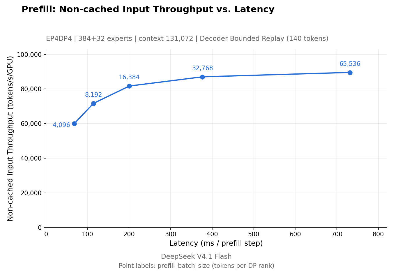
Source: DeepInfer official repository, pinned commit. Four GPUs, 128K context, 140-token bounded replay; the x-axis is a Prefill step, not TTFT. Not re-measured by this article; no precise data points were fabricated from the images.
The x-axis is not a full request's TTFT. Depending on request type and deployment, the time before the first token returns may also include queueing, cache restoration, visual encoding, chunked prefill, and cross-stage transfer. If a long input needs multiple steps, quoting the chart's per-step milliseconds as "128K first-token latency" is switching metric definitions.
Uncached input throughput is also not total logical input throughput. Cache hits can make a service appear to process enormous numbers of history tokens per second, most of which never re-run Prefill. Capacity planning should care about actual newly computed work; business metering may care about logical input. Both can be valid, but they must be booked separately.
The Decode chart contains an explicit acceptance-rate conversion
The official Decode chart uses 64 SM100 GPUs within one scale-up domain, EP64DP64, 384+64 experts, 131,072 context, fixed nextn=3, and a 75% acceptance-rate conversion yielding τ=3.25. plot_pareto.py states the formula directly: τ = 1 + nextn×a, and applies the measured steps/s to both per-user speed and per-GPU throughput.[14][15]
This chart is neither a measurement of dynamic DSpark verification lengths nor a statistic of delivered, billable tokens: it is a device-execution measurement at a fixed-length operating point, converted into an output-speed estimate under an explicit acceptance assumption. The script even refuses to re-apply the formula when variable-length verification is enabled, because that would double-count acceptance.
The a in the formula also needs careful reading. If it denotes the empirical fraction of all proposed drafts finally accepted, then k×a is a reasonable expression for the average number accepted with k fixed drafts; if it is instead read as an identical independent per-position pass probability, the expected prefix length sums a, a², a³… rather than k×a. When citing the chart, keep the authors' declared conversion; do not quietly swap the same "75%" into a different probability definition.
The concurrency labels on the chart are requests per DP rank. With EP64DP64 and CP=1, 64 requests/rank corresponds to 4,096 concurrent requests for the whole group, not 64 for the entire system. This explains how the curve can show high throughput together with degrading interactivity: letting more requests share a step raises total output while lengthening everyone's wait for the next batch of tokens. Different points are not inherently good or bad; the business SLO decides usability.
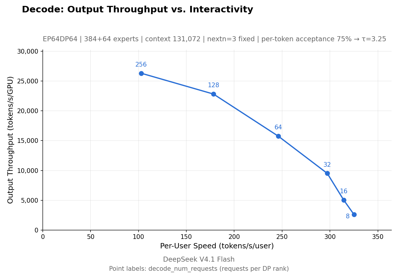
Source: DeepInfer official repository, pinned commit. EP64DP64, 128K context, nextn=3, τ=3.25 at 75% acceptance; not a variable-length DSpark run and not a billable-token measurement. The full correspondence between the original chart's labels and the current default 1017 checkpoint still needs the original run records to confirm.
The benchmark scripts deliberately construct an ideal steady state—know what they exclude
benchmark.py uses random non-special tokens as input, establishes a prefix, then reuses it for subsequent requests; it force-enables the load-balancing path, and the relevant parameters affect the gate's random/balanced routing. Timing separates warm-up from steady state, and intervals overlapping load-statistics refresh are excluded from the "clean" window.[12] This isolates the engine's compute capability, but it does not represent real tasks' expert hot spots, EOS, cancellations, or arrival processes.
Without the original JSONL matching the official charts point for point, one should not eyeball decimals out of a PNG and package them as a precision measurement table. This article keeps the charts' configuration and trends, fabricates no raw data, and declares no speed rankings against other frameworks. The official Wide-EP chart can support "EP64 beats EP8 under the stated conditions"; it cannot, by itself, prove lower cost under fixed total budget, fixed traffic, and equal failure redundancy.[14]
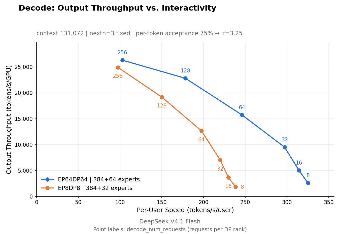
Source: DeepInfer official repository, pinned commit. Group sizes and redundant-expert counts differ; the curves are not a cost experiment at fixed total traffic and fixed total budget.
A correct reproduction has two stages. First, pin repository commit, submodules, checkpoint revision, toolchain, drivers, device model, and topology; reproduce the official sweep with profilers off, and keep all raw results, not just the best-looking chart. Second, switch to real or representative business inputs with normal expert routing, real EOS, actual sampling parameters, and realistic cache lifetimes, and compare no-speculation, fixed-length, and dynamic verification separately.
The second stage should use open-loop arrival loads, or preserve real arrival times. With only fixed closed-loop concurrency, clients automatically send fewer requests as responses slow, which can mask server overload. What to watch is when TTFT, inter-token p95/p99, error rates, and queue lengths lose control as offered load increases—and how much SLO-qualifying output is delivered before that boundary. Speculative output can also arrive in sudden batches; average tokens/s does not describe the streaming experience.
In the end, keep two clocks: one clean steady-state window for explaining kernel and scheduler limits, and one full-service window including cache reads, EPLB re-shuffling, GC, scaling events, failures, and retries. The former finds bottlenecks; only the latter can support procurement and cost decisions.
Eleven: In the Current Inference Ecosystem, What Is DeepInfer Actually Competing With?
Describing DeepInfer as "a faster engine that fully replaces vLLM" is inaccurate. The README itself states it was initially based on vLLM and inspired by SGLang and TensorRT-LLM.[1] Caching, expert parallelism, speculative decoding, and scheduling overlap are not capabilities other projects lack. What is worth comparing is the optimization boundary, the degree of service delivery, model and hardware support, and how much integration responsibility the deployer accepts.
| System | How to position it today | The difference that matters most for selection |
|---|---|---|
| DeepInfer | A public inference core co-designed deeply around DeepSeek models and target hardware | Specialized compute graph, cache semantics, and scheduling coordination; full online service must be completed by the deployer |
| vLLM | An inference and serving ecosystem for broad models and hardware | General access, compatible APIs, tooling, and connectors; specific advanced feature combinations need item-by-item verification |
| SGLang | A runtime and service ecosystem for LLM, multimodal, and agent/RL workloads | Prefix reuse, HiCache, PD, and gateway capabilities fit naturally into system-level comparison |
| TensorRT-LLM | A deeply optimized inference stack on the NVIDIA platform | Integration of hardware features, parallelism, memory, and serving paths; check the support matrix per current version |
| NVIDIA Dynamo | A distributed inference service and control plane, not a same-layer kernel engine | Routing, planning, state transfer, and deployment orchestration; complements engines rather than competing on kernel speed |
This table describes positioning, not a promise that every combination of model, quantization, hardware, PD, and speculative feature is wired up. This article also ran no cross-framework measurement on identical V4.1 weights and hardware, so it offers no speed ranking. The generic capabilities listed do not mean each framework fully supports every feature of this V4.1 checkpoint.[16][17][18][19]
Caching is a good axis for a deeper comparison. SGLang HiCache organizes GPU, instance host memory, and backend storage into tiers, with L1/L2 remaining instance-private and cross-instance sharing determined by the actual L3 backend; DeepSeek's published production design places long-term global KV on dedicated shared storage to ease the conflict between prefix-affinity routing and compute balancing.[2][17] The comparison is between "bring compute to where the cache already is" and "let shared cache support free scheduling". One depends on network and storage capability; the other leans on locality and routing. There is no load-independent universal winner.
PD disaggregation is similar. vLLM's current official documentation still marks disaggregated Prefill as experimental and cautions that disaggregation itself does not guarantee a throughput gain.[16] It can improve the mutual interference between TTFT and Decode tail latency and let the two pools tune independently; it also adds transfer, idle capacity in each pool, deployment granularity, and control-plane complexity. DeepInfer's model compression, Wide-EP, and disaggregated deployment should be attributed separately—not every gain should be booked to "splitting into two machines".
The TensorRT-LLM comparison especially needs shedding stale impressions. As of this verification, the official latest migration documentation states the TensorRT engine backend has been removed, PyTorch is the sole execution backend, and separate checkpoint conversion and engine-build steps are no longer required. Summarizing the current difference as "static precompiled TensorRT versus dynamic Python" is no longer accurate.[18] What needs verifying is the target model's execution path, quantization support, graph and parallelism strategy, and how the service layer exposes them.
Dynamo represents another dimension: organizing different engines into a scalable distributed service. It is more likely to combine with DeepInfer as "control plane plus execution core" than to replace it. We found no official plug-and-play DeepInfer backend, so any integration advice should be treated as an engineering project to implement and test, not a shipped feature.[19]
Twelve: Turning Performance into Money—First Define the Factory's Effective Output
$38 per GPU-hour is revenue, not cost
The official Q&A self-reports one cluster serving 155 trillion tokens per day, achieving $38 per GPU-hour of revenue at valley pricing.[2] That number helps you understand the scale of their operating ambition; it cannot be used to derive GPU rental costs, gross margins, or third-party deployment profits. It also involves input, cached-hit input, output, pricing, and traffic mix—one must not read every logical token as freshly generated Decode tokens billed on the spot.
The numerator of inference cost must cover complete resources, not just busy Decode GPUs. Prefill, visual encoding, draft paths, storage, networking, CPUs, host memory, standby capacity, cold starts and idle time, plus operations and amortized engineering, can all matter. Owned hardware should account for depreciation, capital, and energy; if a cloud rental quote already includes power, stacking the same component again is double billing.
The denominator needs a definition too. This article recommends counting as effective tokens only successfully delivered, deduplicated output that meets pre-agreed quality and latency conditions. Rejected drafts, padding, verification intermediates, cancelled-but-undelivered content, and retried duplicate output do not enter the denominator; the cost spent on them stays in the numerator. If the full service costs C per hour and delivers G effective output tokens per second, then cost per million effective outputs is:
Cost per million effective outputs = C × 1,000,000 ÷ (3,600 × G).
This is an evaluation convention, not a repository-native metric. Quality is best accepted per task; there is no need to pretend every online token can be individually judged correct. Report cost per successful task alongside, so the model cannot inflate the token denominator by simply answering longer. For long-input/short-output applications, also report uncached-input cost and per-request cost, or pure output metrics will mislead.
A transparent example where higher peak, worse economics
Everything below is an assumed example—not a DeepInfer measurement, not a market quote for any GPU. Consider a single Decode pool at $4 per GPU-hour, equal quality, and 95% of output meeting latency requirements. The effective utilization factor expresses how much of a specific benchmark operating point's capacity is realized across the whole paid window; it is not the SM-busy percentage on a GPU panel.
| Assumed scenario | Benchmark output per GPU | Effective utilization | In-SLO output per GPU | USD per million effective outputs |
|---|---|---|---|---|
| A: baseline | 1,000 tokens/s | 60% | 570 tokens/s | 1.95 |
| B: faster, utilization unchanged | 1,500 tokens/s | 60% | 855 tokens/s | 1.30 |
| C: faster, more idle | 1,500 tokens/s | 30% | 427.5 tokens/s | 2.60 |
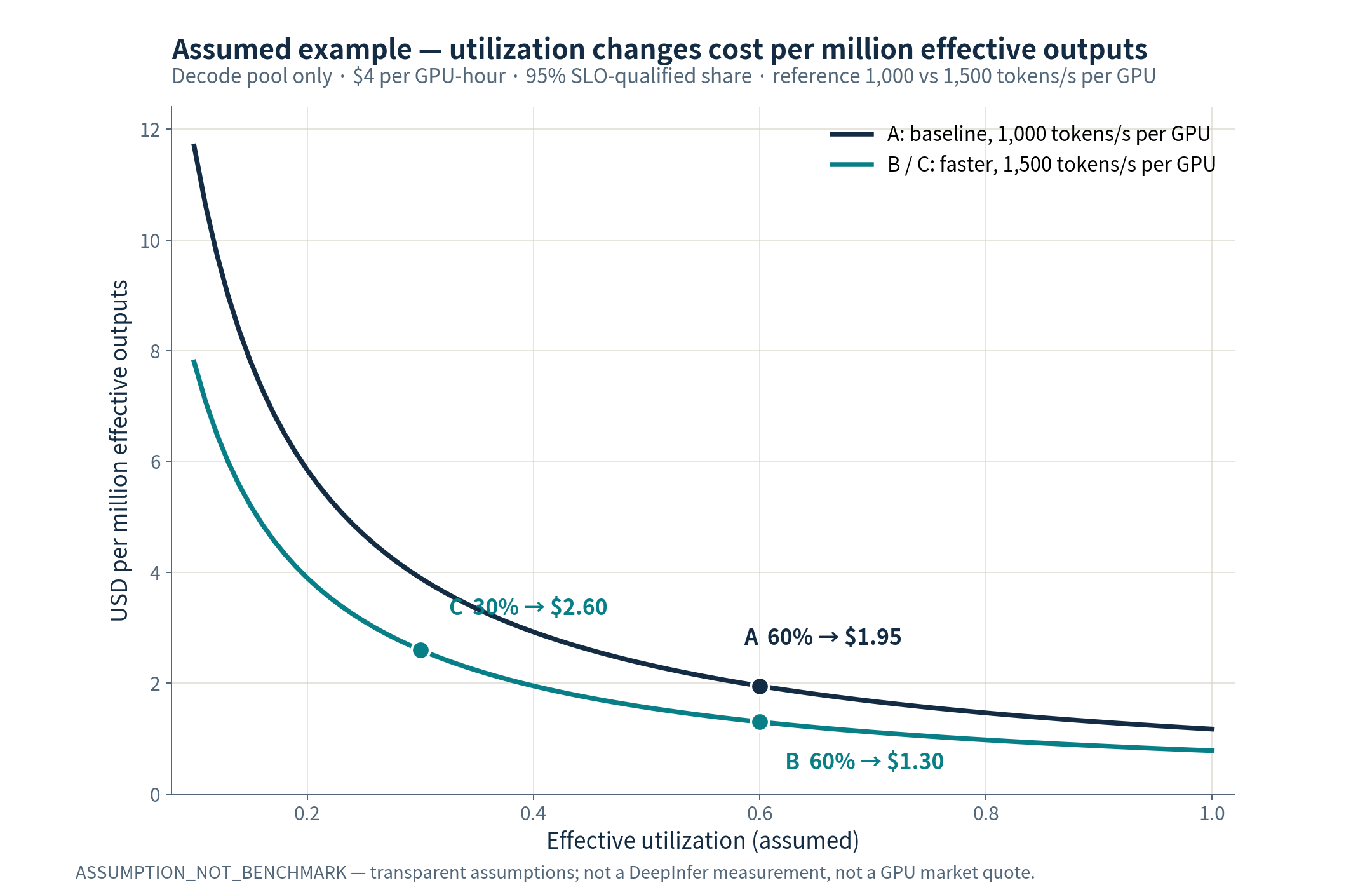
All parameters in the figure are transparent assumptions, not DeepInfer benchmarks or GPU quotes; it models an example Decode pool only and excludes the rest of a full service's costs.
From A to B, unit cost falls by about a third. From A to C, peak is still 50% higher, yet unit cost rises by about a third. Plausible causes of the reversal: EP groups too large, insufficient demand, isolated resource pools unable to lend capacity, or scaling granularity too coarse. A faster core creates room, but the economics only cash in if it releases machines, shortens paid time, cuts energy, or absorbs more SLO-qualifying demand.
If G has already been measured directly over a complete window, do not multiply utilization or acceptance factors again. Those factors exist to extrapolate a full-window output from a partial benchmark; real delivery logs already contain the losses, and subtracting them a second time overstates cost.
Prefill and Decode are serial capacity; the slowest stage ships the factory
Suppose the business needs ρ uncached input tokens per output token; the Prefill pool has Np GPUs at effective uncached throughput Qp each, and the Decode pool has Nd GPUs at effective output throughput Qd each. Ignoring further bottlenecks, raw system output capacity is capped by min(Np×Qp/ρ, Nd×Qd). Vision, storage, and networking can push the ceiling lower still.
This says the P:D resource ratio should track the uncached input/output ratio, each stage's efficiency, and parallelism granularity—not a permanent 1:1. Higher cache hits reduce new Prefill compute but do not automatically shorten the history Decode must attend over; longer outputs push the bottleneck toward Decode. Different businesses on the same model can need entirely different ratios.
One further bottleneck-illustration assumption only: 64P+64D at $4 per GPU-hour each, other costs $128/hour, $640/hour total; Prefill benchmarked at 10,000 uncached input tokens/s per GPU at 50% effective utilization, Decode at 1,000 output tokens/s at 75%, ρ=10. Prefill contributes 32,000 tokens/s of output-equivalent capacity; Decode contributes 48,000; the system is Prefill-bound. Applying a 95% effective-delivery share, cost is about $5.85 per million effective outputs.
At that point, speeding up Decode alone by 50% changes neither total delivery nor this unit cost. Doubling Prefill capacity first moves the bottleneck to Decode, and the example's cost falls to about $3.90. This model ignores queueing and bursts and is not a recommended procurement configuration; it only shows that one stage's speedup cannot be multiplied straight into system-level cost.
Caching, speculation, and migration each have a break-even
Whether to keep a prefix long-term compares its expected future reuse count times the avoided Prefill cost against write, occupancy, matching, read, network, and recovery costs. The longer you keep it, the fewer new hits may arrive while capacity stays occupied. Equal request-level hit rates save entirely different amounts of compute for a 1K hit versus a 100K hit. The more useful metric is "compute avoided per unit of storage cost"; cache capacity by itself says little.
Whether speculative decoding pays compares the cost of a full speculative cycle divided by actually committed length against the per-token cost of the non-speculative baseline. Drafts running on separate devices must be included; a high acceptance rate does not guarantee profit, because total generation-plus-verification time may be longer. Dynamic budgeting is valuable precisely because different operating points want different settings.
Migration has fixed costs too. If one-off integration and migration spend is F and the unit-cost difference between old and new systems at equal quality and service level is Δc, the break-even volume is roughly F/Δc. Assume migration costs $50,000 and saves $0.50 per million effective outputs: about 100 billion effective output tokens are needed to cover the fixed spend, before counting parallel operations and risk. This pure assumption is a reminder: at large enough scale, small-percentage optimizations are worth a lot; below that scale, engineering simplicity and reliable launch may be worth more.
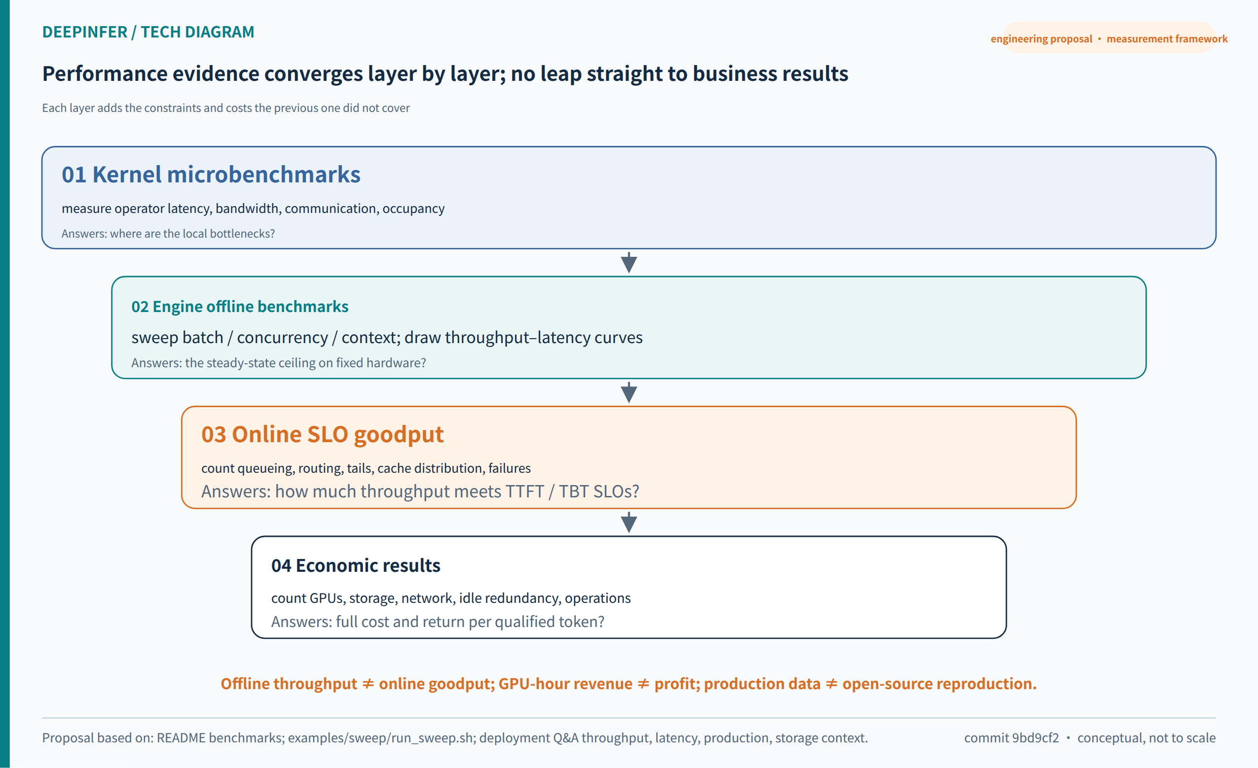
How to read Figure 11: peak performance becomes cost-accountable output only after passing through real load, acceptance, delivery, quality, and latency constraints. A directly measured full-window goodput must not be multiplied again by acceptance or utilization factors.
Thirteen: Extending It into a Production Engine—Build at the Seams, Don't Rewrite Forward
What follows is an engineering route derived from the public code—not a DeepSeek roadmap, and not a promise of a few-week project schedule. The principle is simple: first earn verifiable single-engine reliability, then widen the blast radius of state and failure; secure correctness and resource ownership before chasing cross-node reuse and peak throughput.
Layer 1: the online adapter must be a real lifecycle boundary
The first thing to add is a serving adapter, not another model executor. It should organize a long-running engine loop around add_request, step, abort_request, and output draining, letting external requests arrive asynchronously, be cancelled, and depart; network threads must not block the model step directly, and wrapping synchronous LLM.generate per request is not an online continuous-batching service.[3]
The input side needs authentication, tenant quotaing, request-size limits, deadlines, overload rejection, and an observable wait queue. The output side needs stable events, backpressure, client-disconnect handling, and deduplication. After a request is cancelled, "queued but not executed", "executing on device", "sampled but unsent", and "sent but not yet metered" are different states, each needing defined resource-release and accounting responsibility.
DeepSeek Recipe can carry the conversion between Chat Completions, Responses, Messages and a unified internal session representation, plus template encoding and streaming-output parsing. But its README explicitly leaves inference, tool execution, and HTTP transport to the caller; it is not a complete API server.[20] Its handling of special tokens is valuable: template-inserted control tokens are encoded differently from identical-looking user text, and output recognizes control boundaries by true token IDs. That reduces control-token injection without solving every semantic prompt-injection or tool-security problem.
Structured output should also get a resource boundary here. DeepInfer constrains output with grammar compilation and sampling masks rather than a final JSON check. The compilation cache must be bounded; schema size, complexity, compile time, and tenant quota all need limits, or an innocuous-looking feature becomes a CPU, memory, and latency attack surface. Format validity is still not business correctness: tool names, parameter permissions, and business validation remain application responsibilities.[21]
Layer 2: treat cache as a versioned, permissioned, owned data service
Define an explicit CacheManager contract—match, fetch, commit, abort. These names are this article's proposal, not existing public APIs. match returns the reusable prefix and state availability; fetch asynchronously retrieves compatible data; commit publishes only completed, fully readable cache; abort reclaims unfinished writes and leases. External I/O can attach at existing points—post_schedule, do_save_kvcache, Prefill save hooks—rather than wedging blocking storage calls into every layer's forward.[3]
A cache key cannot be just a text hash. It must bind at least weight revision, tokenizer and template version, precision and layout version, full prefix identity, multimodal-input or embedding identity, plus an authorization namespace. The same text's state from different model versions may be incompatible, and identical prefixes across tenants must not auto-share visible content. Cross-tenant reuse requires an explicit public-content and permission policy first.
Cache transfer must verify integrity, record source–destination layout negotiation, and protect in-use blocks with leases or reference counts. During rolling model upgrades, old and new layouts coexisting cannot be judged compatible because "dimensions look alike". On storage timeout or metadata pointing at dead objects, the system needs a controlled fallback: recompute safely, or explicitly refuse under resource pressure—never load partial state and keep generating.
Block KV and SWA state also need separate promises. A global prefix hit does not mean SWA is simultaneously available; a missing SWA should enter bounded replay by design, and recovery must not overwrite existing long-term global KV. Wrapping both into one opaque cache file makes invalidation policy, transfer optimization, and quality diagnosis harder.
Layer 3: P/D transfer needs a protocol, not a memcpy
Once single-engine serving is stable, evaluate E/P/D disaggregation. Set up a dedicated TransferManager with explicit export, import, ack, and cancellation semantics. After Prefill completes, when does Decode take request ownership? When may the source release KV? If the destination fails mid-import, will a retry duplicate generation? If the user cancels mid-transfer, who reclaims state on both sides? A protocol must answer these—normal-path execution order is not an answer.
Request ID plus execution epoch distinguishes old attempts from new. Receivers should be able to judge whether late data, late outputs, or completion notices are stale; a request ID alone cannot prevent post-retry confusion. For tool calls already streamed out, retry must not cause downstream double execution. Deduplicating model-service output and deduplicating tool side effects are connected but distinct responsibility boundaries.
Transfer must also consider layout compatibility across differing P/D EP configurations. Different parallel sizes across pools do not mean caches can be copied in the same buffer layout. Layer-wise loads that can overlap, metadata that must complete early, and state that must survive until verification ends should all enter an explicit event protocol and its tests.
Layer 4: the control plane schedules cost and deadlines, not just request counts
Prefill routing should know uncached input volume and existing context; Decode routing should weigh concurrency and total KV length together. Two requests both being "one request" does not mean they occupy equal resources. The official internal design—Prefill allocating by context bucket, Decode balancing request count and KV length jointly—is a concrete instance of this kind of resource estimation.[2]
But the load model must also be calibrated by the business. Over-pursuing cluster throughput can starve large requests indefinitely; over-favoring short requests can starve high-value long-context tasks. Production scheduling needs deadlines, tenant fairness, and overload policy—explicitly stating which SLOs win—not just a throughput-maximization formula.
Scaling should observe vision, Prefill, Decode, and storage separately, not treat one tier's metric as system-wide demand. Drain before shrinking; in-flight long requests may migrate or wait within set resource and time bounds; Wide-EP's minimum granularity and standby capacity decide how much ideal elasticity is actually realizable. If considering a control plane like Dynamo, adapters, events, and metrics protocols come first—the tool cannot be assumed to understand DeepInfer's StateBlock and speculative state automatically.
Layer 5: acceptance centers on failure paths, not one successful demo run
The repository already ships tests for sequences, sampling, state caching, expert rebalancing, batch invariance, offline long inputs, and distributed cases, plus model-eval and YOCO-equivalence scripts. The reasonable move is to extend from this base, not to describe the project as untested.[6][22]
Numerical correctness should be verified in layers. Batch invariance concerns model computation across batching combinations; deterministic sampling further requires fixed random streams and configuration—the README gives the NVIDIA path with DEEPINFER_BATCH_INVARIANT=1, MTP varlen disabled, and a fixed seq_seed. None of these automatically proves identical output across different cache-hit points, approximate recovery modes, or hardware.[1]
More pointedly, the LLMEngine.step source explicitly notes that with YOCO truncation enabled, preemption may change results. Production acceptance should therefore cover "before/after preemption", "before/after cache-miss recovery", and "cold cache versus warm cache" task quality, and must not treat passing batch-invariance tests as proof of full semantic stability.[3] For factual retrieval, evidence citation, and long-program editing, small average-score differences can hide concrete failure modes.
The table below compresses the route into executable acceptance gates. It does not demand that every team build every capability; it demands that a team know which new risk it is taking on before entering the next layer.
| Build stage | Results that must be proven | Typical stress or fault injection |
|---|---|---|
| Pinned versions and baseline | Output, quality, and timing reproducible on target hardware | Precision/config switches, long context, varying batches |
| Single-engine online service | Cancellation, backpressure, metering, draining correct | Slow SSE clients, disconnects, timeouts, duplicate requests |
| Distributed cache | No tenant crossover, no version mixing, failures fall back safely | Wrong keys, truncated objects, stale directory, storage jitter |
| E/P/D disaggregation | State ownership and retry semantics explicit | Mid-transfer link cut, late ack, destination restart |
| Cluster scheduling and elasticity | Sustained in-SLO goodput | Bursts, long/short mix, hot experts, shrink-induced tails |
| Production acceptance | Cost benefit holds with all resources counted | GPU failure, cache-miss storm, rolling upgrade |
Each stage should retain p50/p95/p99, error rates, cancellation rates, real committed tokens, cache-hit lengths, state-load times, speculation verification and acceptance counts, and the slowest-rank/average-rank ratio. Time and resources spent on failed requests must not be deleted from cost samples. Only when the system remains cheaper and steadier under these conditions has a specialized optimization become production capability.
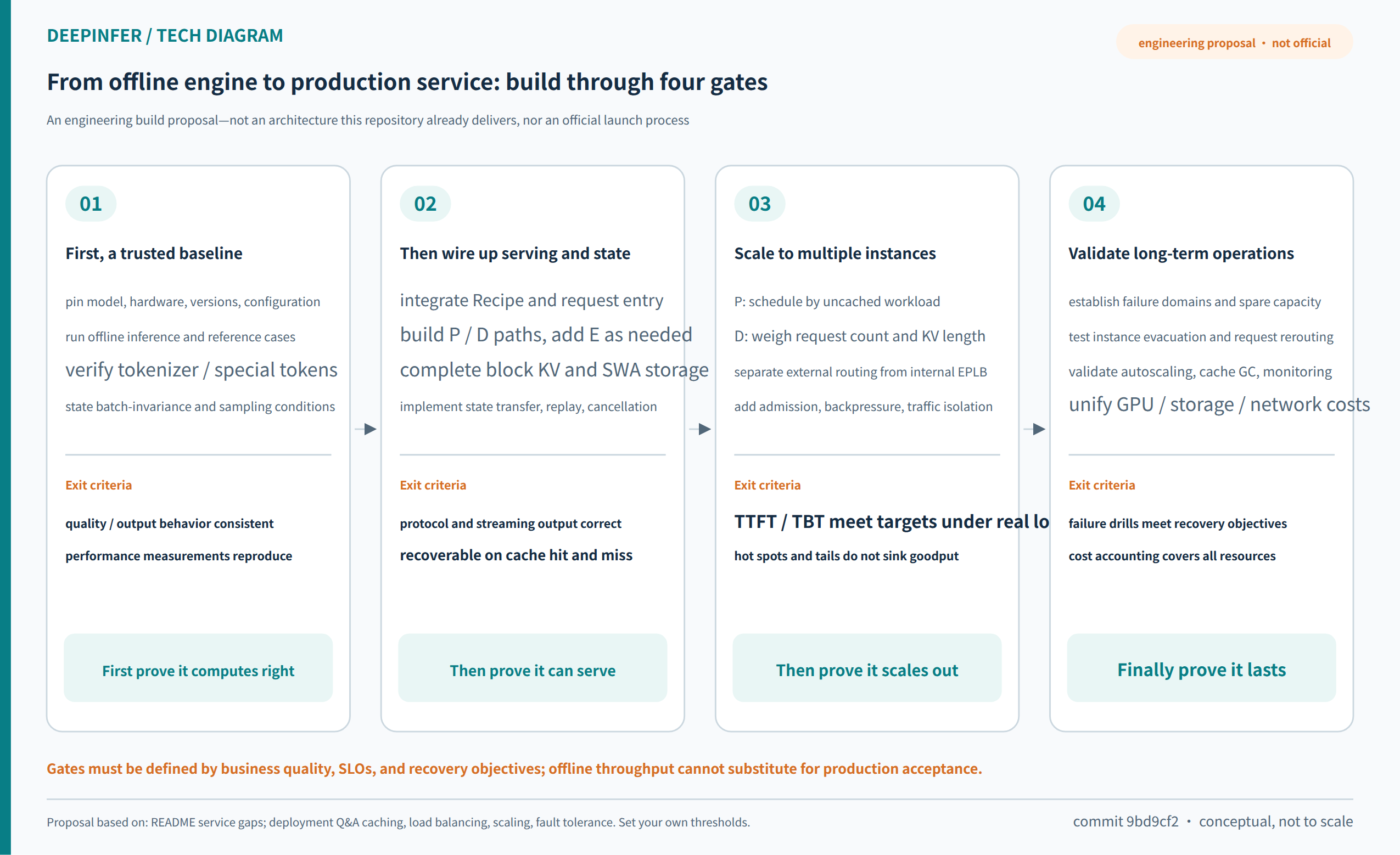
How to read Figure 12: interface integration, cache correctness, transfer protocol, and the control plane are incrementally widening risk boundaries; the route is this article's engineering proposal, not an official implemented-feature list or release-date promise.
Fourteen: What to Watch Next—The Next Competition May Not Be in a Single Kernel
DeepSeek has stated that future models' inference code and follow-up performance work will continue to be opened in DeepInfer.[2] That is a direction statement; it includes no specific open-sourcing timeline for a complete KV store, load balancer, or other integration components. Based on the existing design, the directions worth tracking can be made concrete—but they must be labeled analysis, not promises.
First, models will keep writing system cost into structure and training. CED, cross-layer KV sharing, hierarchical indexing, and training-adapted bounded replay show that model design already optimizes beyond per-token FLOPs—toward state retention, cross-machine movement, and long-horizon reuse. Future optimization may organize more directly around "how long is a historical state still worth reading", but reducing state cannot bypass task-quality validation.
Second, scheduling will consume more model-produced information. DSpark's Confidence is one example: the model produces not only text but signals that can guide resource allocation. The next step worth studying is folding confidence, deadlines, context cost, and tenant service classes into one budget—while preventing throughput-chasing algorithms from sacrificing the few hard requests. The smarter the optimizer, the more calibration, explainability, and fallback policy matter.
Third, multi-hardware support will move from "can run" toward "shared semantics with independently verifiable performance". Different devices differ in operators, communication, memory, and numerics; flattening all differences behind one abstraction may sacrifice efficiency, while fully forking multiplies maintenance. DeepInfer's platform layer plus specialized kernels is a live specimen of where that balance lands.
Fourth, Wide-EP elasticity and failure recovery may become the crux of operating at scale. Large domains make steady state more efficient—and make low-load fragmentation and single-point failures more expensive. If parallel sizes can change more smoothly, with requests migrated and experts redistributed, the payoff may rival shaving another few percent off a kernel. But these capabilities entangle state, topology, and correctness; they are not a one-parameter change.
Fifth, specialized engines and general ecosystems need not be enemies. General frameworks offer model breadth, interfaces, and integration experience; specialized implementations validate more aggressive co-design, and effective ideas can flow back into common components. DeepInfer's most durable influence may be proving which interfaces should be open, which state can be separated, and which approximations are worth training in—not just the fastest execution path for one model generation.
Conclusion: Whether to Use It Depends on Which Segment of the Value Chain You Are Prepared to Carry
If you operate a large-scale token factory—business concentrated on DeepSeek, suitable scale-up interconnect, and the ability to build caching, routing, and failure handling—DeepInfer deserves serious production candidacy. The right starting point is not a promise to reproduce official revenue, but pinning business quality and SLOs and verifying that co-design's savings actually cover the added storage, network, redundancy, and engineering. The target worth chasing is lower cost per successful task and more predictable delivery, not higher offline tokens/s.
If you are building an enterprise multi-model platform with modest traffic, shifting requirements, and a premium on time-to-launch, general frameworks usually offer the better default landing point. DeepInfer can serve as a dedicated model pool or performance lab without migrating all serving into a more specialized, more self-built system for one model's peak. Low-load efficiency, version maintenance, and replaceability are real cost advantages too.
If you are an infrastructure vendor, the opportunity is mostly not "rewriting forward once more" but productizing this class of efficient cores: versioned caches, compatible transfer, reliable streaming interfaces, SLO scheduling, multi-hardware acceptance, failure recovery, and auditable metering. The distance between an open core and a full production system is not a missing-feature list; it is a systems-engineering effort that can become a product moat.
DeepInfer's most important lesson is putting model structure, numeric precision, cache lifetimes, communication topology, speculative budgets, and service economics into one design sheet. First reduce the work not worth doing; then execute what remains efficiently; finally prove it actually turned into good results users received. That is the full path from an inference engine to a token factory.
Sources and Verification Notes
All DeepInfer code links in this article are pinned to commit 9bd9cf243fc53ef9afbf8f04d391d989117d6ab9 so later main-branch changes cannot silently alter the conclusions. The model report and other framework documentation were verified as of October 23, 2026; unpinned pages may continue to change. Official production scale, revenue, TTL, and performance disclosures are self-reported by the source and were not independently re-measured here. Cost examples and custom diagrams are analysis tools, not observations.
- DeepInfer README: release scope, supported platforms, configuration.
- DeepSeek V4.1 Flash Inference Deployment Q&A.
- LLMEngine: request lifecycle, extension hooks, async resource management. Related entries: LLM.generate; local cache: CacheEngine / StateBlock; block lifecycle: BlockManager.
- C++ Scheduler: open scheduling and chunked-Prefill path.
- DeepSeek-V4.1-Flash Technical Report. This article relies on §2.2–2.4, §3.2, the parameter configuration, and the limitations discussion; model info can be cross-checked against the official model card.
- YOCO mask/compact equivalence test notes.
- EPLB policy: physical expert replicas and load placement.
- MoE/MLP: Mega-MoE enabling conditions and fused path.
- MTPVarlen: verification budget, performance curves, runtime estimation. Related implementations: drafting and Confidence, GPU budget allocation.
- Worker: async forward, sampling, and post-processing timing. Related implementation: ZOS metadata correction.
- SharedLayerTopology: cross-layer KV and index sharing.
- benchmark.py: input, routing, and timing methodology.
- Platform: GPU/NPU adaptation.
- Official performance charts: Prefill, Decode, and Wide-EP. Originals: Prefill, Decode, Wide-EP.
- plot_pareto.py: throughput and acceptance-rate conversion. Reproduction entry point: run_sweep.sh.
- vLLM: disaggregated-Prefill boundary and connectors. General capabilities: vLLM repository.
- SGLang HiCache: cache tiers and sharing boundary. See also the SGLang repository and PD disaggregation.
- TensorRT-LLM: current backend migration notes. Migration statement cross-checked against the official source docs; feature support must be checked against the model support matrix.
- NVIDIA Dynamo: distributed inference runtime architecture.
- DeepSeek Recipe: protocol, encoding, and streaming-parse boundaries.
- Structured output compiler: compilation and cache configuration. Runtime constraints: Sampler.
- DeepInfer test directory. See also the evaluation notes and offline examples.
- KV format definitions: FP4 main KV, indexer, SWA.
- Engram runtime: hashing, sharded lookup, gated fusion. The mHC correspondence is in mhc_modeling.py; structural claims follow the technical report.