
Walking one expert-parallel round trip end to end
Abstract: Measuring MoE communication by GB/s alone is not enough; four things must be tested separately:
- Bandwidth: the official five tiers decline monotonically from EP8 to EP128;
- Padding: in this piece’s constructed example, alignment padding brings processed slots to three times the valid data;
- Load: under synchronous execution, a stage’s duration is set by the last device to finish;
- Overlap: overlap gains depend on dependency structure and resource contention; to measure them, device execution streams, communication streams, and host-side issue and wait must be put on one timeline.
With the four measured separately, the same bandwidth can correspond to an end-to-end result that actually explains itself.
Part 2 left a question at grouped matrix multiplication: the busiest expert’s m_i and the waiting structure deserve their own look. The reason is simple: when several stages must synchronize, the whole segment’s duration is set by the last device to finish. The busiest device is not necessarily the slowest, but the slowest one holds up the whole segment.
This part leaves the single chip and, following DeepEP-Ascend’s public interfaces, walks one MoE layer’s token round trip end to end. The questions to answer: when the buffer is created, reused, and destroyed; at which step the data lands; where the waiting happens. Once the path is walked, the four observation dimensions of communication optimization each map onto concrete steps.
1. The Full Timeline of One Round Trip: From Routing to Merge
One MoE layer’s round trip has three segments:
- dispatch: group each token’s input by routing result and send it to the experts’ devices;
- expert computation: grouped matrix multiplication on the expert side;
- combine: merge the weighted results back into the original requests.
The buffer: long-lived, created once, reused repeatedly. The three segments are not initiated ad hoc; they are organized around a long-lived EPBuffer (DeepEP README):
- one buffer per expert-parallel group, reused across layers and microbatches;
- construction fixes each rank’s maximum token capacity, hidden size, and top-k; all ranks’ capacities must agree;
- buffer pools can be planned with
get_buffer_size_hint. After all uses and waits finish, buffers are destroyed explicitly.
Why must capacities agree? This is all-to-all: each rank’s receive buffer must hold everything peers might send at the capacity limit. If one side underestimates, the other side’s limit-rate data has nowhere to land.
dispatch: returns immediately. Training, prefill, and decode share one set of interfaces. Calling buffer.dispatch passes this rank’s input x, the routing result topk_idx (fixed int64) and weights, plus a few parameters that decide execution shape:
expert_alignment: must match the grouped GEMM’s token alignment;do_expand: expand data into the expert-side layout;do_zero_padding: pad zeros to the alignment granularity;do_cpu_sync: can be turned off when the expert kernel uses device-side counts directly, saving one CPU synchronization;async_with_compute_streamanddefer_epilogue: make communication asynchronous to the current compute stream.
The call returns a pending object immediately.
The standard usage is itself an interleaved schedule. The README’s standard usage is: initiate the communication, run the computation independent of it, and wait only when the results are needed. In the example, the shared expert sits between dispatch and wait. The steps:
- wait returns the received inputs, routing information, and a handle. The handle records this dispatch’s grouping and counting structure; backpropagation will reuse it during training.
- The expert side’s grouped matrix multiplication consumes the received data; Part 2’s alignment agreement takes effect here. The routing weights
recv_weightsare applied once on this compute path. - Results go to
buffer.combine. What is merged is the already-weighted results, with the shared expert’s output added in as bias. - Wait again; the final output arrives.
The timeline of one round trip is therefore:
routing → dispatch (async) → [shared expert and other independent compute] → wait (inputs + handle)
     → grouped GEMM (apply routing weights) → combine (async, merge weighted results, bias = shared output)
     → wait → output
Compare this with Part 1’s component map and the interface design shows through. dispatch and combine can both be issued first and waited on later; the gap in between is for the user to schedule independent computation. The handle preserves the dispatch’s routing relations for combine and backpropagation. Communication and computation are not “first one, then the other”; they are a set of interleaveable operations, controlled explicitly by wait timing.
2. issue, drain, epilogue: The Boundary of Timing and Waiting
The official bandwidth table notes: timings include issue and drain, and exclude the final epilogue (DeepEP README). The three words cover three pieces of work:
- issue: submitting the communication kernel;
- drain: completing the data movement;
- epilogue: the finishing work. Per the official implementation,
defer_epiloguepostpones both “host waiting for receive counts” and “copy finishing” to the event wait, not just one compute kernel.
Device-side waiting is wait()’s job. It makes the current stream wait on recorded events and schedules the finishing work into the current stream; subsequent operators on the same stream read results in order. This dependency binds only the current stream. It guarantees in-order results downstream on this stream; it does not mean the CPU has waited out all device work. Another stream needing this data must synchronize across streams first.
Host-side waiting is a different matter. do_cpu_sync only synchronizes receive counts back to the CPU, not the same kind of waiting as the stream dependency above. When this switch is worth turning off is covered at the end of this section.
This boundary matters both to measurement and to engineering.
For measurement. The bandwidth figures exclude the epilogue. Estimating whole-layer latency by dividing communication volume by the table’s bandwidth misses the finishing work and the waiting. Comparing two implementations requires checking which stages each side’s timing covers, for example whether finishing is counted. This is the same class of question as Part 6’s metric definitions.
For engineering. First the buffer itself: while any operation is outstanding, the buffer cannot be resized, reused, or destroyed. Reusing a buffer requires its previous communication to have fully completed. If different layers’ communications are in flight simultaneously, give them separate storage and separate lifecycle management, rather than freeing one buffer early by reordering waits.
Then the handle’s cross-segment reuse. The handle records this dispatch’s routing and counting structure; combine and backpropagation both use it. Within one training step the handle is reused many times; before each reuse, the communication it belongs to must have completed. Which wait goes first is arranged around this requirement.
do_cpu_sync applies the same idea to counting. By default, the token counts received by each expert are synchronized back to the CPU. If the expert kernel uses device-side counts directly, this step can be turned off; the host need not make a dedicated synchronization just to learn “how many rows each expert received.” A small switch, but it removes one pipeline stall.
3. Four Observation Dimensions: Look Again After Walking the Path
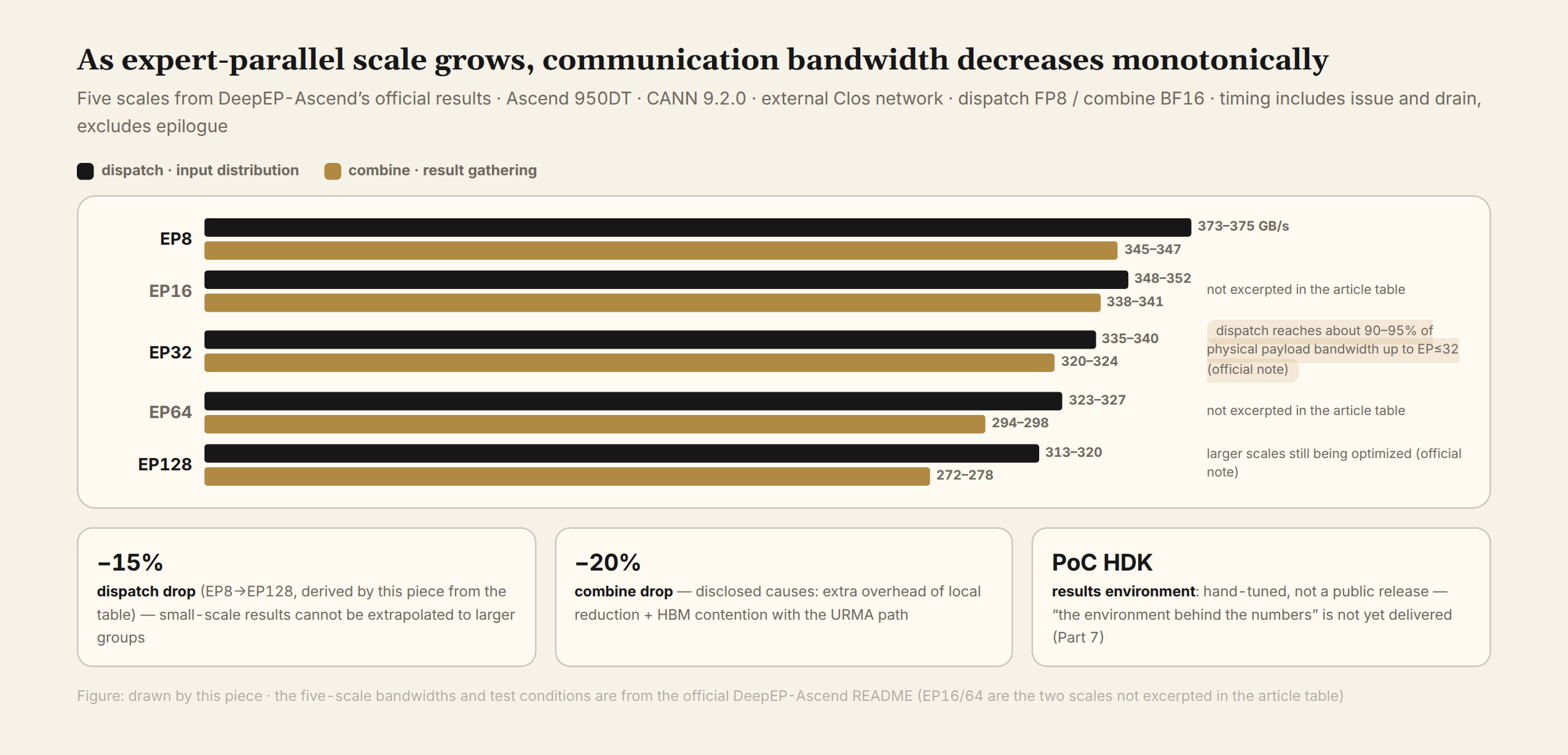
With the path in hand, the official five-tier bandwidth table can be read in full. Test conditions (DeepEP README):
- hardware and software: Ascend 950DT, CANN 9.2.0, the manually configured PoC HDK;
- network: the external Clos network (supernode’s netlayer 1);
- load: 16,384 tokens per rank capacity, hidden size 7168, 256 experts, top-6;
- resources and configuration: 32 AI Cores / 64 vector cores (official wording: 32 AI cores / 64 AIVs), expert alignment 128, no bias;
- precision: dispatch in FP8, combine in BF16;
- sampling: 10 warmups and 50 samples per tier, with cache flushing.
| Expert-parallel size | Dispatch | Combine |
|---|---|---|
| EP8 | 373–375 GB/s | 345–347 GB/s |
| EP16 | 348–352 GB/s | 338–341 GB/s |
| EP32 | 335–340 GB/s | 320–324 GB/s |
| EP64 | 323–327 GB/s | 294–298 GB/s |
| EP128 | 313–320 GB/s | 272–278 GB/s |
All five tiers decline monotonically. By this piece’s estimate from the table, dispatch drops about 15% and combine about 20% from EP8 to EP128. The README explains part of the reason: for EP sizes up to 32, sustained dispatch reaches roughly 90–95% of the physical payload bandwidth; combine is lower partly from local-reduction overhead and partly from HBM contention on the URMA path. Larger sizes remain under optimization.
Bandwidth is only the first dimension. The other three, put back on the path:
Padding. Section 1’s do_zero_padding is where Part 2’s padding cost actually occurs. Take alignment granularity 128: three experts receiving 1, 1, and 126 tokens each pad up to 128, occupying 384 slots. Valid data is 128 rows, one third. As a padding amplification factor A_pad (processed slots ÷ valid rows), A_pad = 3 here. The more fragments, the more groups fall below the granularity and the worse the amplification; the exact amount is computed from actual rows and granularity. The same fragmented distribution often both lowers arithmetic intensity and raises padding.
Load. Under synchronous execution, if four devices need 10, 10, 10, and 30 ms, the stage takes nearly 30 ms, not the 15 ms average. Speeding up the first three does not shorten the critical path. Diagnose by pairing each device’s token count with its latency:
- the slowest device genuinely holds more tokens, is always the same one, and correlates with placement: only then adjust placement;
- similar token counts but very different latencies: check device state and execution path first;
- the slowest device rotates with requests: again compare token counts and latencies. Only when the load rotates too does it point to routing volatility; “the slow device changes” alone does not.
Overlap. Section 1’s timeline is overlap at the interface level, but “supports async” does not mean the gain is realized. Let communication take 40 ms and parallelizable computation 60 ms: ideal overlap approaches 60 ms total. If running both together causes contention, computation stretches to 80 ms and communication to 70 ms; the overlapped segment is set by the slower computation. Total is about 80 + h, where h is the tail that comes after computation and cannot be covered by overlap, a parameter assumed by this piece. Only when h is under 20 ms does overlap still beat the 100 ms serial baseline.
Whether the gain materializes depends on dependency structure and contention. Put device execution streams, communication streams, and host-side issue and wait on one timeline; measure the actual overlap and contention; thread ordering alone is not enough. The README says “async is supported”; the numbers have to be measured.
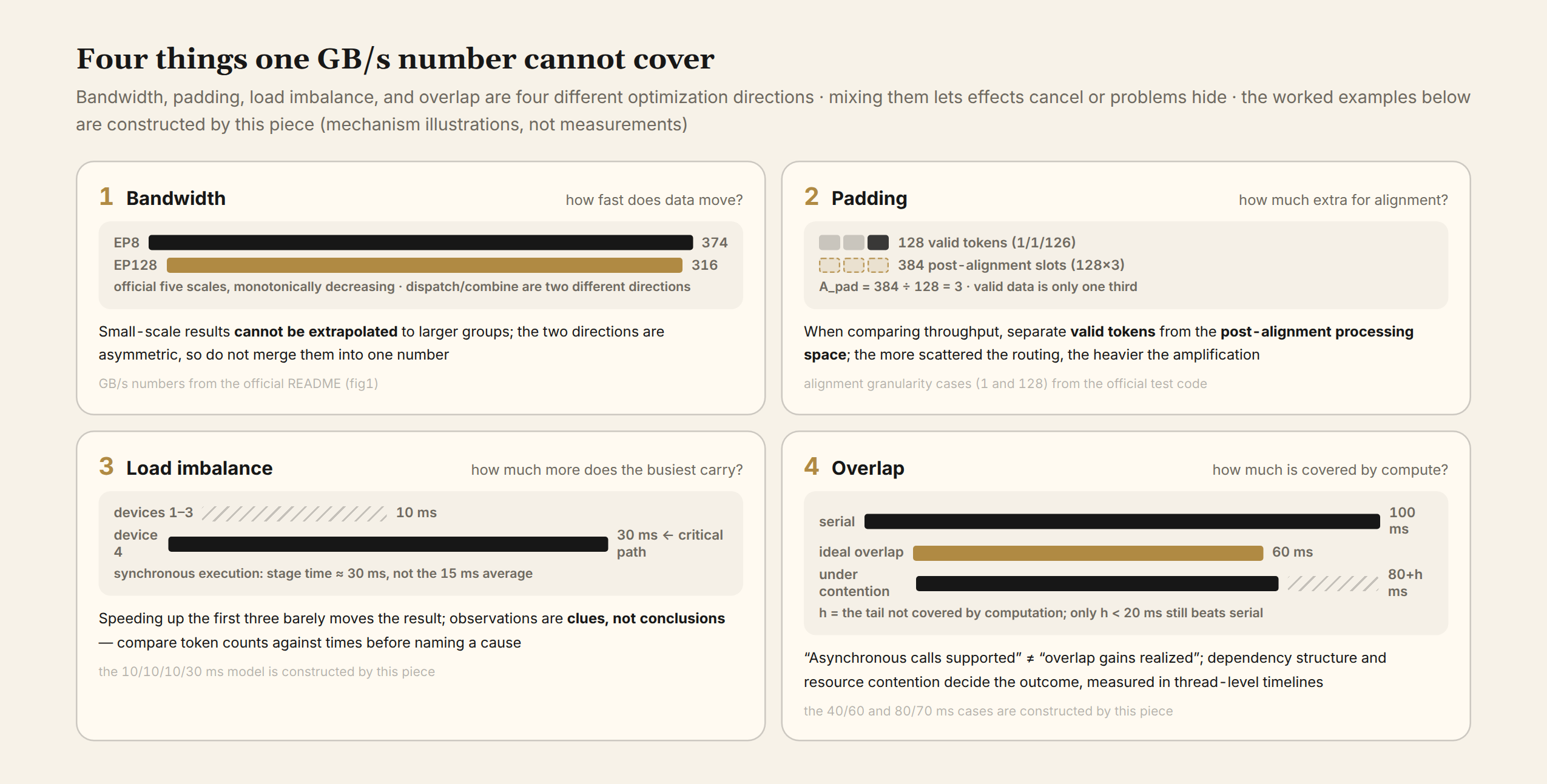
Taken together, the question stops being “is the bandwidth high” and becomes: under the real routing distribution and compute load, how much communication time remains on the critical path.
4. What Still Separates the Public Conditions from the Full Path
Read the interface list in full to see what a framework must still supply (DeepEP README):
| Status | Contents |
|---|---|
| Usable | EP dispatch/combine, with constraints: do_expand and allow_multiple_reduction must be True, do_handle_copy must stay False, routing indices int64. num_sms selects the AI Core count on Ascend. Cached dispatch/combine reuse the counts saved in the handle |
| In development | Bucket collectives: batched all-gather available; reduce-scatter and all-reduce kernels still in development. Expert load balancing: lb_prefetch_weights, lb_reduce_grads expose aligned APIs; Ascend communication kernels not yet implemented |
| Experimental | PP, Engram |
| Explicitly unsupported | mixed communication, CPU-side Engram storage, graph capture |
This list reads the same way as Part 1’s: interface alignment is not capability alignment.
- An inference framework wanting to put the whole execution into CUDA-Graph-style capture hits an impassable limit in unsupported graph capture;
- A parallel strategy depending on reduce-scatter must decide, given the Bucket gap, whether to wait for the kernel or route around it.
One more environmental fact belongs in the comparison conditions: these results come from a manually configured PoC HDK, not a public release. Part 7 folds the distance between “the code reads” and “the results reproduce” into the ecosystem judgment.
The next part returns inside the chip, to the most eye-catching performance number in this release: FlashMLA’s sparse attention, and the data-supply trade-offs behind 95% peak utilization.
Sources and computation notes: This piece is based on DeepEP-Ascend’s public repository and official test code, fact-checked as of October 7, 2026, with a pinned copy kept. From the official README: the EPBuffer lifecycle; dispatch/combine interfaces and parameter semantics; the “initiate communication, run independent compute, then wait” usage; the five-tier bandwidth table and all test conditions (including the official wording 32 AI cores / 64 AIVs); “timings include issue/drain, exclude epilogue”; and the capability tiers and in-development list. The two alignment cases (1 and 128) come from the official test code. Constructed or derived by this piece: the padding example (1/1/126 → 384 slots, A_pad=3); the 10/10/10/30 ms load model; the 40/60 and 80/70 ms overlap counterexample; and the EP8 → EP128 declines (about 15%/20%). “Capacity agreement exists so the receiving side can hold what peers send” is this piece’s reading of the requirement. No hardware measurements were made. This is Part 3 of the DeepSeek Ascend open-source series.