
Through DeepGEMM: data layouts, matrix shapes, and performance boundaries
Abstract: API compatibility reduces the rework at the calling layer. Integration cost is decided by data layout; performance gain by real matrix shapes; the three must be assessed separately. On Ascend, UE8M0 scaling factors are packed pairwise into int16, so mathematically equivalent computation must be stored differently in memory. Under the same N and K, M=128 and M=4096 reach 549 and 861 TFLOPS respectively. This piece also constructs a counterexample: kernel time down 30%, the whole segment 5% slower. Evaluation should compare what can be handed downstream directly.
The previous part concluded: migration is rearranging the relations among computation, data, and resources. This part goes one level down with a single question: when a matrix-multiplication library claims “API compatibility,” where does the real cost of replacement sit? Answering it means following the interface all the way down: how data is arranged in memory, what shape matrices enter the kernel with, and what the kernel does to keep the hardware fully loaded.
“API compatibility” has value, but which layer is compatible must be settled first. Identical function names and parameter positions mean calling code may survive. They do not guarantee that the tensor’s internal data arrangement, quantization scaling factors, or execution cost are also identical. DeepGEMM-Ascend happens to be an example that carries this all the way through.
1. Which Layer Is Compatible: How Scaling Factors Are Laid Out in Memory
DeepGEMM-Ascend’s README states that the scaling-factor format on Ascend differs from the NVIDIA version: every two UE8M0 factors along K are packed into one int16, stored MN-major for best hardware efficiency, and the repository provides a layout-conversion tool (DeepGEMM README).
Notation first. This piece writes matrix multiplication as A(M×K) × B(K×N) = C(M×N):
- M, N are the rows and columns of the output C. Scaling factors are organized along MN: A’s factors by row, B’s by column.
- K is the contraction dimension summed over after multiplication. One scaling factor per 32 K elements.
- UE8M0 is a factor format storing only the 8-bit exponent. “Packed pairwise” means two adjacent 8-bit factors along K share one 16-bit word.
“MN-major” does not mean “contiguous along K”; it is the opposite. Take A’s factors (B is analogous, with the axis swapped to N): let MN=2 (rows a and b), K=128, one factor per 32 K elements; each row has four factors a0…a3 and b0…b3. Packed pairwise, each row keeps two int16s in a 2×2 layout, MN-axis stride 1, K-pair-axis stride 2:
| K pair 0 (k0–63) | K pair 1 (k64–127) | |
|---|---|---|
| row a | (a0, a1) | (a2, a3) |
| row b | (b0, b1) | (b2, b3) |
The in-memory order is (a0,a1), (b0,b1), (a2,a3), (b2,b3). That is, the factor pairs of both rows at the same K position sit adjacent. Reading one row along K, say row a from (a0,a1) to (a2,a3), every next pair skips over the intervening pairs of other rows; adjacent K pairs of the same row are not contiguous in memory. This is exactly the reverse of “each row’s own factor pairs stored contiguously.” One mathematical object, two storage orders, each suiting kernels that read in a different order.
So a real new step appears beneath interface compatibility. The layout produced upstream by the quantization operator may not match the layout the kernel requires. But conversion does not happen every time: the layout tool first checks whether the existing layout already satisfies the requirement, and reuses it directly if so. When the conversion happens decides where the cost is booked:
- Fixed weights convert once at load time, booked as startup cost;
- Per-layer activations, if they need conversion, book into every request’s running time.
The repository’s transform_sf_into_required_layout tool hands exactly this cost decision to the user.
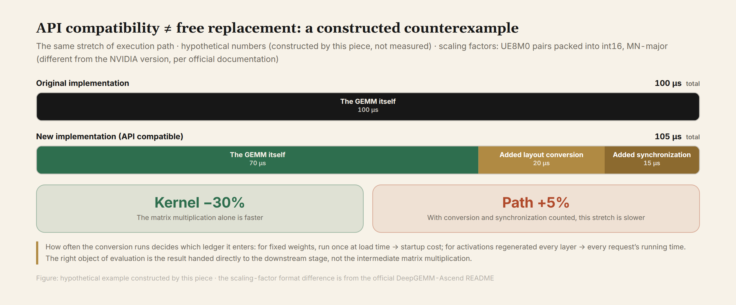
A purely hypothetical swap example can be constructed to show the trap in evaluation:
| Item | Original | New |
|---|---|---|
| GEMM itself | 100 µs | 70 µs |
| New layout conversion | 0 | 20 µs |
| New synchronization | 0 | 15 µs |
| Total | 100 µs | 105 µs |
The new GEMM itself is 30% faster, but with conversion and synchronization counted in, this segment is 5% slower. This does not mean the kernel optimization is worthless; it means the evaluation target was wrong: compare what can be handed downstream directly, not the intermediate matrix multiplication alone. The table is this piece’s constructed counterexample, not any measurement; its purpose is to put “which bills remain after compatibility” on the table.
2. Matrix Shape: From Formula to a Real Computation
DeepGEMM-Ascend’s public FP8 inference benchmarks cover seven (N, K) shapes and two M tiers. Conditions: Ascend 950DT, CANN 9.2.0, cold L2, timed with bench_msprof (DeepGEMM README). Take the N=7168, K=16384 tier:
| M | Latency | Compute | Memory bandwidth |
|---|---|---|---|
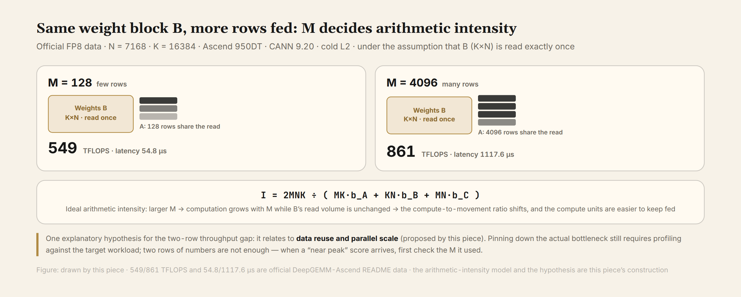
| 128 | 54.8 µs | 549 TFLOPS | 2456 GB/s |
| 4096 | 1117.6 µs | 861 TFLOPS | 186 GB/s |
Two intuitions fail on this table:
- The second row is not less efficient because it takes longer; it processes a bigger matrix.
- Nor can every request get 861 TFLOPS just because that row is higher. The rows are different shapes; what shapes actually appear in service is decided by batching and routing.
The most informative column is memory bandwidth: 2456 GB/s at M=128, only 186 GB/s at M=4096. That is not regression; the shape changed the ratio between computation and data movement.
An ideal model makes this computable. Assumptions and formulas first, for C(M×N) = A(M×K) × B(K×N):
- computation is about F = 2MNK;
- assume each input element is read once and each output written once, FP8 inputs at 1 byte, BF16 output at 2 bytes: minimum data D = MK×1 + KN×1 + MN×2;
- ideal arithmetic intensity I = F/D.
Substituting M=128: F ≈ 3.01 × 10¹⁰ FLOP, D ≈ 121.4 MB, I ≈ 248 FLOP/byte. Weight B’s KN bytes are spread over only 128 rows; each byte moved supports about 250 operations. By this model, saturating the official 865 TFLOPS ceiling at this shape would need about 3.5 TB/s of sustained bandwidth.
Substituting M=4096: D ≈ 243.3 MB, I ≈ 3954 FLOP/byte. The same weights spread over 4096 rows; saturating compute needs only about 0.22 TB/s. The official measurement is 861 TFLOPS, 99.5% of the 865 TFLOPS hardware ceiling.
The gap between the two rows is thereby explained: larger M amortizes weight reads.
One reading restriction remains. To judge which resource the M=128 tier is actually bound by, the table’s 2456 GB/s cannot be used directly: it shares its origin with throughput, the official statistics dividing tensor bytes by the same duration, so it cannot serve as an independent bandwidth ceiling. A related caution: dividing this piece’s D by the official latencies yields deviations in both directions: about 2215 GB/s versus 2456 at M=128, and about 218 versus 186 at M=4096. The official byte accounting (whether scaling factors are counted, which output precision) does not fully match this piece’s D assumptions, and the README does not publish the details; the official GB/s is used only as a same-origin statistic, the model D only to explain shape trends, and the two are not interchanged. Where a performance number comes from and what a bottleneck judgment is based on are two different things.
This is also why “near peak” must always be asked about together with shape. Given any TFLOPS figure, first check its M, then check how M distributes in your own service, to know which band you can land in. When comparing benchmarks, also check the conditions implicit in the table:
- data type: tables split FP4×FP4, FP8×FP4, FP8×FP8, and BF16;
- cache state: cold L2;
- tool and software versions.
With a warm cache or a different precision, the same shape’s bandwidth and throughput both move.
3. Grouped Matrix Multiplication: After Routing, Shape Follows Distribution
In the MoE setting, the shape problem is amplified. Let a batch hold 1024 tokens; each token picks k experts by routing and sends one copy to each chosen expert. The expert side then receives token-count × k input rows in total, and the rows expert i receives are its m_i.
Describing expert computation as a distribution (m_1, m_2, …, m_E) carries more information than “1024 tokens total.” E is the expert count; under top-k routing Σm_i = token total × k (the equality assumes no token is dropped or truncated by capacity). Two batches with equal totals may concentrate rows on a few experts or spread them evenly across all.
Grouped matrix multiplication (M-grouped GEMM) exists for exactly this input: each expert’s input matrix is one group, and multiple groups merge into one kernel call. The official benchmark table gives two tiers with large average rows per group:
- 4 groups, 8192 rows per group on average;
- 8 groups, 4096 rows per group on average.
These two tiers reach 818–862 TFLOPS compute with only 98–180 GB/s of memory bandwidth. Weight reads are fully amortized by large row counts; the top tier approaches the 865 TFLOPS compute ceiling.
Read the table strictly by its header. The README states “M per group” is the average number of tokens received per group. So:
- large average rows are the benchmark configuration’s choice, not the real routing distribution;
- the average also hides imbalance between groups;
- small, fragmented m_i push the shape toward the low-arithmetic-intensity end.
To judge which resource a given distribution is actually bound by, first estimate computation and movement with Section 2’s model and the real row counts, then check against independent resource limits and measured data. The in-table GB/s shares its origin with throughput and cannot serve as independent bandwidth evidence. The busiest expert’s m_i and the waiting structure are analyzed separately with Part 3’s method.
Distribution also ties into alignment. DeepEP’s dispatch carries an expert_alignment parameter whose README comment says it must “match the grouped GEMM’s token alignment.” DeepGEMM provides tools for group-level M/K alignment under contiguous layouts, alongside the theoretical minimum. The routing output distribution, the communication-side padding alignment, and the kernel’s grouped shape are three contracts on one execution path.
A fragmented row distribution both lowers arithmetic intensity and pushes more groups below the alignment granularity, adding padding; whether it adds, and how much, is computed from actual rows and the alignment granularity. Low arithmetic intensity and heavy padding often come from the same fragmented distribution.
4. One Level Further Down: The MAD Abstraction and Kernel Pipelines
The last layer of “why replacement cannot just rename functions” is the kernel implementation itself. The README positions the library as “a lightweight abstraction over Ascend MAD (matrix multiply-add) primitives,” hiding fractal layouts, alignment constraints, address calculation, and low-level parameters to keep GEMM kernels concise, while “making extensive use of sparse data loading and coroutine-based pipelining” to approach hardware limits (DeepGEMM README).
Each of the three statements corresponds to something concrete:
- Fractal layout is the data organization Ascend’s matrix unit requires. Upper-layer code reads matrices by rows and columns; the hardware consumes fractal blocks. The re-shuffling in between is another instance of “mathematically equivalent, different in memory,” like Section 1’s scaling factors, only this time done by the library beneath the interface.
- Sparse data loading (the README’s wording) is a named optimization direction whose public description does not expand the implementation. Part 4 shows the complete form of “move only the selected data” in an attention kernel; whether the two use the same technique is not asserted here.
- Coroutine pipelining means the kernel internally organizes movement and computation into interleaveable stages; software pipelining schedules which stage waits for data and which produces results. It is the same idea as Part 3’s dispatch/combine overlap at the stream level, applied at a different granularity.
The abstraction hides this complexity inside the library, with two consequences: kernel authors write less and tune more precisely; users do not see the layout re-shuffling and more easily mistake “same API” for “same execution model.”
The surrounding tools are therefore worth reading as an adaptation checklist:
- layout conversion: settles Section 1’s bill;
set_num_sms: caps the AI Cores available to the kernel (the official term is AI cores; the name reuses NVIDIA’s SM);- determinism switch: the README does not document its mechanism;
- cross-validation tests against aclnn reference implementations, for the corresponding GEMM interfaces; coverage per the test code, expanded in Part 5.
So, API compatibility reduces calling-layer rework; data layout decides integration cost; real matrix shapes decide performance gain; the kernel abstraction decides what “compatible” really means. Assess the four separately, and only then does the replacement decision have a basis.
The next part leaves the single-machine view and walks one expert-parallel round trip end to end: how tokens are dispatched, how buffers are reused, where the waiting hides.
Sources and computation notes: This piece is based on DeepGEMM-Ascend’s public repository, fact-checked as of October 7, 2026, with a pinned copy kept. Scaling-factor formats, surrounding tools, the MAD abstraction wording, and the benchmark tables come from the official README, official results under Ascend 950DT, CANN 9.2.0, cold L2, bench_msprof. Section 1’s layout example parameters and memory order follow the official tests’ actual stride checks on outputs (commit 8491bbb4); “check first whether a layout can be reused” follows csrc/apis/layout.hpp. Section 1’s swap counterexample (100/70/20/15 µs) is constructed by this piece. Section 2’s D, I, and the sustained bandwidths needed to saturate 865 TFLOPS (about 3.5/0.22 TB/s) are this piece’s computation under FP8 inputs, BF16 outputs, and single read/write per element; the official GB/s byte accounting does not fully match this piece’s D (both deviation directions noted in the text) and is not used as an independent bandwidth ceiling. expert_alignment “matching the grouped GEMM’s token alignment” is from a DeepEP README comment. No hardware measurements were made. This is Part 2 of the DeepSeek Ascend open-source series.