

Taking the design trade-offs behind 95% apart, item by item
Abstract: FlashMLA’s official 410/360 TFLOPS are sparse attention results measured under their own declared workload conditions. Behind the numbers sit three kinds of arrangement with different natures:
- Compute less: sparse selection reduces the attention items computed per query; this piece derives from the 2,048-of-131,072 setting;
- Move less: on-chip tiled computation and accumulation cut the round trips of intermediates between device memory and on-chip storage; the online softmax state lives on this layer;
- Pack tighter: the execution pipeline, including 64-head grouping per core, the 1C2V ratio, and the UB-transfer supply line, decides how fast the work completes.
Each arrangement reduces one kind of work and has its own conditions. After the input shape changes, performance cannot be inferred from peak utilization.
FlashMLA’s officially published results: Prefill up to 410 TFLOPS, Decoding up to 360 TFLOPS, reaching 95% and 83% of hardware peak respectively (README and Ascend technical report).
The percentage alone says little. It shows the compute resources are heavily used; it does not show what arrangements the implementation made to get there. This part follows the official technical report’s chain of decisions step by step (Ascend Prefill deep-dive report). The starting point is what state the algorithm must maintain; then four design questions are answered in turn:
- how many heads each AI Core processes;
- where the output accumulator lives;
- how many vector cores to use;
- which path the data takes into the Cube core.
Finally, how these decisions compose into one pipeline. Walk the chain, and “fast” stops being just a number.
1. Starting Point: What the Algorithm Itself Must Maintain
This kernel computes the forward pass of DeepSeek Sparse Attention (DSA). Following an index table, each q token attends only to the “most important” selected KV positions. For a single q token, computation has four steps:
- gather KV by the index, producing
gathered_kv; - compute scores P = QKᵀ;
- compute S = softmax(P ×
sm_scale); - compute out = S·V.
Meet the parts that recur below.
- AI Core: the compute unit on Ascend. Each AI Core has one Cube core for matrix multiplication and vector cores for element-wise computation and data-movement assistance.
- L1: the input buffer before data enters the Cube core.
- L0C: the dedicated accumulation buffer on the Cube side.
- UB (unified buffer): on the vector side.
- MTE2: the path moving data from device memory into on-chip storage.
- FixPipe: the dedicated path moving L0C results out to UB.
Section 5’s supply-line figure draws the full data path. This section needs only one fact: results in L0C must go through FixPipe to leave.
Online softmax: process in blocks, maintain global state. Softmax needs the whole row, while KV is processed in blocks of B_TOPK selected positions (usually 64 or 96). The implementation therefore uses online softmax, same family as Flash Attention, maintaining four states throughout, all float32:
running_max: the row maximum;running_max_for_softmax: the reference maximum used for scaling;running_sumexp: the sum of exponentials;out_accum: the output accumulator.
The final output is normalized by the accumulated sum of exponentials.
skip-scale: do not rescale until the threshold. Rescaling has a trigger threshold. Only when the true maximum exceeds the current scaling reference maximum by more than the threshold (usually 6 in the kernel) is the scale recomputed. The reason: old accumulations were obtained under the old reference maximum and must be multiplied by exp(old reference maximum − new maximum) to align with the new scale. Absent the trigger, this rescale is skipped, and the current block’s sum of exponentials, SV multiplication, and output accumulation proceed as usual. This is skip-scale.
The trick pays off unusually well on NPUs, for a reason that recurs below. If the output accumulator sits in L0C on the Cube side, scaling cannot happen in place: it must go through FixPipe to UB and be multiplied there by a vector core. Every rescale pays this path. Section 3 shows the final design pinning the accumulator in UB for exactly this reason.
Skipping rescale saves more than computation: it saves FixPipe, UB, and vector-core bandwidth, plus power. Only when power drops can the clock rise. One algorithm-layer judgment directly changes which resources the execution layer spends.
2. How Many Heads per Core: Where the Number 64 Comes From
The first design question: how many q heads does each AI Core process? The report gives a model you can compute along with.
- Compute side: a fully loaded Cube core does 4096 FMAs per core per cycle.
- Memory side: total L2 bandwidth 5 TB/s, divided by 32 cores and 1650 MHz, is about 95 bytes per core per cycle.
Let head count be h_q, selected positions topk, dimension d = 512. Computing, for one head group, all selected positions of a single q token:
matrix compute cycles ≈ h_q × topk × 2d ÷ 4096
              (one QKᵀ plus one SV)

data movement cycles ≈ (h_q × d × 4 + topk × d × 2) ÷ bytes per core per cycle (~95)
              (Q reads and output writes at 2 bytes each; KV read once)
These cycle counts are totals over the whole span of selected positions; Section 1’s B_TOPK is only the loop block size.
Substituting four head counts (memory cycles computed at the unrounded ~94.7 bytes per cycle):
| h_q | topk | Compute cycles | Memory cycles |
|---|---|---|---|
| 16 | 512 | 2,048 | 5,883 |
| 32 | 1024 | 8,192 | 11,765 |
| 64 | 1024 | 16,384 | 12,457 |
| 128 | 1024 | 32,768 | 13,841 |
Note: the report gives complete data for each head count at both topk=512 and topk=1024; this table takes the 512 tier for the first row and the 1024 tier for the rest, all values verbatim from the report, and the rows are for reading the trend, not same-condition comparison.
The pattern is clear:
- below 64 heads: memory cycles far exceed compute cycles; the kernel is bandwidth-bound;
- at 64 heads: compute cycles have passed memory cycles (16,384 versus 12,457), the two are fairly close, and the transition sits near 64;
- above 64 heads: compute cycles exceed memory cycles by more and more, and duration is increasingly decided by computation.
Why not 128 heads? Two hardware facts block it:
- L0C cannot hold it. The 128-head output accumulation matrix is 128 × 512 × 4 bytes = 256 KB and would occupy L0C by itself. The accumulator would have to move to the vector side, with two vector cores running a fine-grained “move a stretch, accumulate a stretch” pipeline, which the report calls extremely hard to write.
- Throughput would not rise. Microbenchmarks show that 64 rows of MMAD already saturate the Cube core; 128 heads bring no higher throughput.
So 64 heads became the design point: right at the memory-compute transition, and right where the Cube core starts to saturate.
3. Where the Accumulator Lives: L0C Cannot Scale In Place
Online softmax raises the next design question directly: where does the output accumulator live? A hardware constraint stands in the way: data in L0C can only leave through FixPipe or serve the Cube core as an accumulator; it cannot be multiplied by a scalar in place. And rescaling is exactly multiplying the accumulated output by a factor.
The report compares two options:
- Option one: the accumulator stays fixed in UB on the vector side. Partial results the Cube core computes per block stay in L0C, are moved via FixPipe to UB when needed, and added into the UB accumulator.
- Option two: the accumulator stays on the Cube side. When scaling is needed, the accumulated results go via FixPipe to the vector side, are multiplied by the scaling factor, and are put back into the Cube core; the put-back borrows a “multiply by the identity matrix” matrix multiplication.
Option two’s cost can be computed exactly. The put-back is one 64×64×512 float matrix multiplication. Precision requirements force HF32 off, leaving the Cube core 256 FMAs per cycle, so this step costs 8,192 cycles; by this piece’s conversion, about eight times one block’s main computation (~1024 cycles), entirely unacceptable. Note that the 256 FMAs per cycle here is the throughput of a float matrix multiplication with HF32 off; it is not the same workload as Section 2’s 4096-FMA full load, and the two cannot be compared directly.
The final choice is option one: the accumulator lives in UB.
Looking back at Section 1, skip-scale saves exactly the “FixPipe move-out plus vector accumulation” path. The two designs meet here. Triggering one fewer rescale at the algorithm layer saves one move-and-accumulate at the hardware layer; pinning the accumulator in UB means the rescales that must happen no longer need the put-back into the Cube core.
4. Why Two Vector Cores: Three Resources, Each Insufficient
Each AI Core on Ascend 950 has one Cube core and two vector cores. If the kernel used only one vector core (1C1V), the other could run other model modules or cross-device communication, and machine-wide MFU would look better. The report rejected this. Three resources each fall short, and each suffices on its own:
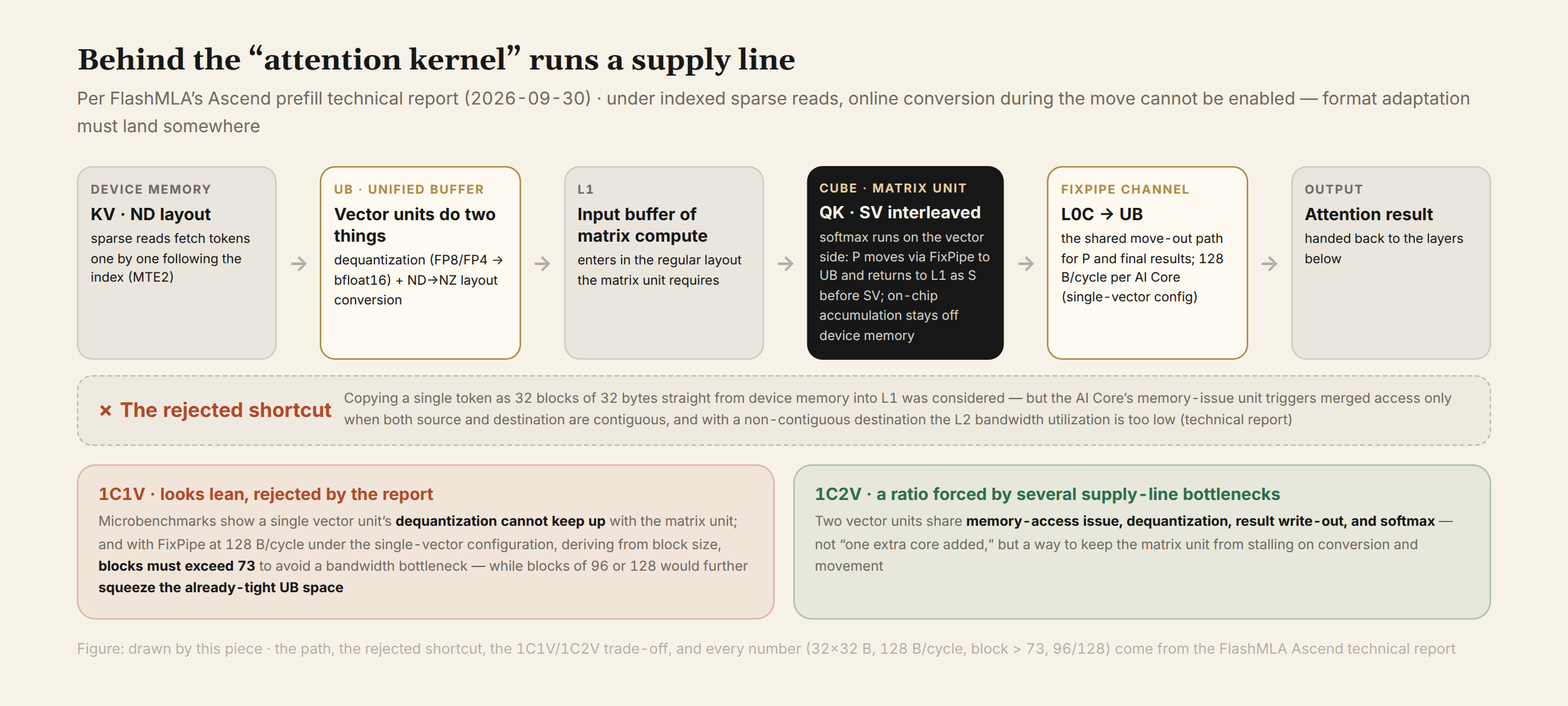
First, the MTE2 issue queue. A single vector core has at most 16 MTE2 copy requests in flight. Even with the gather2 merging described in Section 5, only 32 tokens are in flight, far too few for a kernel that reads sparsely token by token.
Second, dequantization. Decoding must recover bfloat16 from the FP8/FP4 KV cache before feeding the Cube core. Microbenchmarks show a single vector core’s dequantization cannot keep up with the Cube core’s consumption.
Third, FixPipe. With one vector core, FixPipe moves at most 128 bytes per core per cycle. At 64 heads, each block’s matrix-multiply cycles are B_TOPK × 16 and FixPipe transfer cycles are 1024 + B_TOPK × 2; keeping FixPipe off the bottleneck requires B_TOPK > 73.14. Taking 96 or 128 satisfies it but crowds the already tight UB and aggravates the first queue problem.
Three reasons point to one conclusion: 1C2V, two vector cores sharing MTE2 issue, dequantization, FixPipe move-out, and softmax. This is not “one extra core added”; it is a ratio forced jointly by multiple bottlenecks on the supply line.
5. The Supply Line: Which Path the Data Takes into the Cube Core
The parts needed have all appeared; now connect them into the full path.
The problem: mismatched layouts. KV is stored in ND layout in device memory; the Cube core requires NZ (fractal) layout. The usual fix converts on the way from device memory into L1. But this kernel’s KV is moved sparsely token by token, leaving no way to convert in transit.
The rejected shortcut. The report tried splitting a single token (512 bfloat16 values) into 32 blocks of 32 bytes and copying them straight into L1. But the BIU unit that issues memory access merges only when both source and destination are contiguous; the destination is laid out at a stride of B_TOPK × 32B, not contiguous, L2 bandwidth utilization fell too low, and the bottleneck immediately landed on L2.
The final path: through UB.
device memory (ND) ─ MTE2 sparse reads → UB (vector cores dequantize; SIMD vector core does ND→NZ)
                  ─ MTE3 → L1 → Cube core → L0C ─ FixPipe → UB
Several optimizations on this path target “per-token sparsity” specifically:
- gather2. One MTE2 request per token would quickly exceed the 16-deep queue. So
burst_countis set to 2 and the source stride to the distance between two tokens’ start addresses; one request moves two tokens. Copy parameters are computed on the fly by the SIMD vector core, without blocking the scalar core. - The decoding-stage KV layout. The old FlashMLA KV block put all tokens’ data first and all scales after, costing two MTE2 moves per token; this kernel stores each token’s data and scale adjacent, one move.
- The ND→NZ conversion itself. loadalign reads, strided writes; the output buffer pads one extra row to avoid UB bank conflicts; auto-increment pointers remove address-update overhead; adjacent 256-byte pairs are processed at once, keeping all banks working. The report says the conversion finally reaches UB peak read/write throughput.
So an attention kernel was never just two matrix multiplies. QKᵀ, softmax, SV, and output accumulation interleave on-chip. Behind every block of data the Cube core consumes lies a supply line of reads, buffering, dequantization, and layout conversion.
6. Pipelining: Scheduling the Waits into the Timetable
The design is now settled: 64 heads, 1C2V, accumulator in UB, KV via UB. The final layer is pipeline scheduling, with one goal: keep the Cube core busy. The Cube-side basic schedule:
P[i] = Q·K[i]ᵀ → O += S[i−1]·V[i−1] → P[i+1] → O += S[i]·V[i] → …
The previous block’s SV is deliberately delayed. P[i] is computed in the first step but consumed in the fourth, leaving about 1024 cycles in between (at B_TOPK=64, QKᵀ and SV each take about 512 cycles; at 96 the gap is proportionally longer). That window is exactly enough for three things: FixPipe moves P[i] from L0C to UB, the vector core finishes softmax, and S[i] goes back to L1. The wait did not vanish; it was scheduled into the timetable.
The vector side schedules more densely. At any moment it handles work from five different blocks:
- reading the indices of block i+5;
- converting and copying UB→L1 for block i+3;
- computing softmax for block i+1;
- scaling the output O for block i;
- synchronizing the skip-scale signal.
The complexity comes mainly from two hardware facts:
- the skip-scale signal is produced by the SIMD vector core, but the SS buffer, a buffer only the scalar core can read and write, passes the signal via cross-core flags; handled poorly, this becomes one blocking synchronization.
- the hardware pipeline issues instructions in order; one vector instruction stalled on an unmet condition stops the whole PIPE_V with it.
So the schedule must arrange every instruction’s issue order carefully to keep all units busy.
Two more details that reduce idle time:
- the instruction cache is small (Cube 32K, vector 16K, SIMD 8K, in KB). Code must use hardware loop instructions to hold down size and limit inlining.
- L1 has two banks. Splitting a tensor half-and-half across the banks uses both sides’ bandwidth at once.
7. Three Improvements of Different Natures, Each with Its Own Boundary
Beyond the headline numbers, the three improvements must be kept apart.
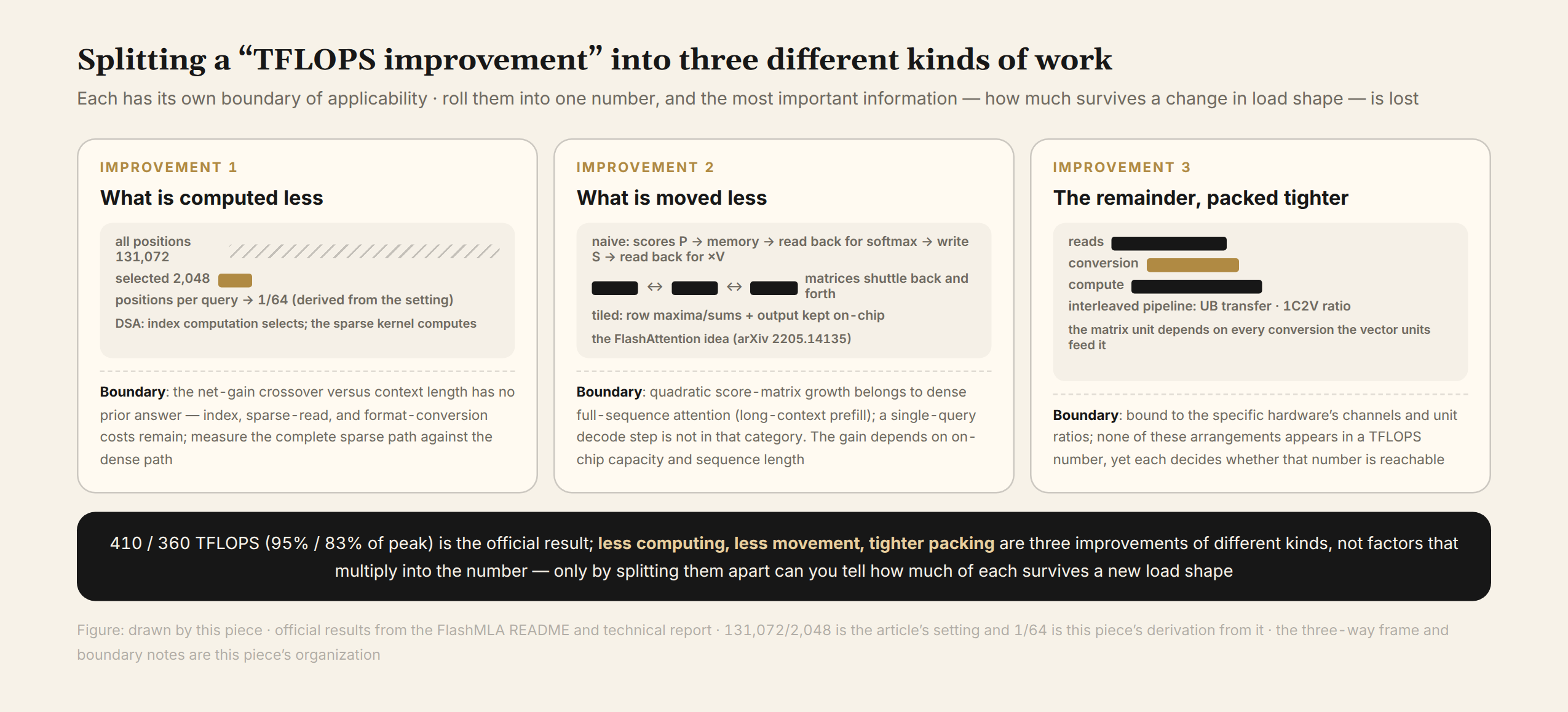
First the setting. Sparse selection shrinks the positions each query must process from 131,072 to 2,048, one sixty-fourth (this piece’s derivation from that setting). This states only the ratio of selected positions, a workload setting. The 410/360 TFLOPS are a different thing: the sparse attention throughput measured officially under their respective declared workload conditions (the README marks the model as DeepSeek-V4.1). A workload ratio cannot be converted into a throughput ratio, still less an overall speedup.
The three improvements, their effects and boundaries:
- Compute less: position selection. It reduces the attention items computed per query. How much time it actually saves depends on how the extra costs of index computation and format conversion grow with context length. The saved computation minus these costs is the net gain, and the official numbers do not give that difference.
- Move less: tiling and on-chip accumulation. Section 1’s online softmax state lives on this layer. Intermediates no longer round-trip device memory; data streams through on-chip storage block by block, with no need to load the whole sequence at once. How much traffic is saved depends on the block size the on-chip capacity allows, the sequence length, and data reuse.
- Pack tighter: the execution pipeline. All the arrangements of Sections 2 through 6. They depend on the unit ratios, path widths, and queue depths described here; a different workload shape requires re-measurement.
When the shape changes, the three do not move in step. Reporting only “TFLOPS improved” discards exactly that information.
The next part leaves performance for a quieter question: when everything appears to run normally, how do you discover that the migration has already gone wrong?
Sources and computation notes: This piece is based on FlashMLA’s public repository and the Ascend technical report, fact-checked as of October 7, 2026, with a pinned copy kept. The 410/360 TFLOPS (95%/83% of peak) and the V4.1 workload note come from the official README; all design decisions expanded in the text come from the official deep-dive report; Section 2’s cycle table uses the report’s own values (the report contains the complete data at both topk=512/1024; the text table is an excerpt, noted as such). The DSA split into indexing and sparse attention comes from V3.2-Exp public materials. 1/64 is this piece’s derivation from the 2,048-of-131,072 setting; “8,192 cycles is about eight times one block’s main computation” is this piece’s conversion at B_TOPK=64. No hardware measurements were made. This is Part 4 of the DeepSeek Ascend open-source series.