Throughput Up 20%, Why Might Cost Rise?

From kernel throughput to service capacity to effective output

Abstract: The unit for comparing performance is not how many tokens per second a device processes, but how much effective work each unit of cost completes under the same business constraints.

Kernel throughput is not service capacity: with the same configuration, tokens 64 → 256 move MegaMoE from 266 to 659 TFLOPS;

Cost can reverse: in this piece’s constructed example, B is 20% cheaper in resources with 20% higher raw throughput, yet costs about 5.6% more per unit of effective output; the break-even line sits near a 63.3% compliant share;

Count the whole bill: one-time investment and recurring maintenance enter the payback period, and each part’s technical choices land on different cost lines.

The first five parts counted the technical ledger: resources, layouts, communication, attention, correctness. This part counts the economic one and puts the technical choices back into service objectives. Before counting, two questions must be settled: what unit to compare with, and what “throughput” refers to at each layer.

The conclusion first: the unit of performance comparison is not tokens per second per device, but how much effective work per unit of cost under the same business constraints.

1. Align the Metric Definitions First

Before comparing, confirm both sides measure the same thing. Take the client-side measurement definitions of the vLLM benchmark documentation:

TTFT: time from sending the request to receiving the first streamed output;
TPOT: per-request average per-token latency, excluding the first token;
ITL: the interval between two consecutive streamed outputs.

All three are called “latency,” but their windows and exclusions differ. If one streamed output carries multiple tokens, ITL and TPOT are not interchangeable. The vLLM documentation itself warns: metric terminology across benchmark tools is not standardized; compare measurement points and formulas, not names.

2. Kernel Throughput Is Not Service Capacity

The deeper problem: these metrics measure service-layer outcomes, while requests pass through one more conversion before becoming the shapes operators actually process.

Request length decides prefill computation and KV volume;
the arrival process decides queuing and bursts;
batching and expert routing decide the input rows of matrix multiplications. For a fixed model layer, N and K are set by that layer’s feature dimensions and matrix definitions and do not change with request volume; what batching and routing actually change is the input rows, in MoE the m_i each expert group receives. Part 2 computed how directly rows change the throughput a kernel can reach.
KV cache capacity decides whether new requests can still be admitted.

So, kernel throughput is a number measured at a fixed shape; service capacity must be measured end to end under given request lengths, arrival process, scheduling, and cache conditions. Intra- and inter-batch interactions, queuing, scheduling, KV capacity, and caching all pull capacity away from any simple weighting of kernel numbers.

This is not abstract. In MegaMoE’s official benchmarks, holding the configuration fixed (96 experts, hidden 7168) and raising only the token count from 64 to 256 moves compute throughput from 266 to 659 TFLOPS (DeepGEMM README; the table does not mark a precision configuration). The kernel’s “throughput” is itself a function of token volume. Treating kernel peak as service capacity assumes the service’s shape forever stays at the benchmark point.

3. Cost Reversal and the Break-even Line

With definitions settled, the full account can be computed. All numbers below are hypothetical and correspond to no hardware quotation. Two options serve the same business at the same quality requirement:

Item	Option A	Option B
Total running cost per hour	100 yuan	80 yuan
Raw output throughput	10,000 Token/s	12,000 Token/s
Token share from compliant requests	95%	60%

Define “compliant” first. A request is compliant only if it meets both the task’s quality requirement and the preset latency requirement. Sum the tokens output by compliant requests and divide by the same observation window: the compliant output, called “effective output” below. Failed and timed-out requests still consume resources and enter running costs and request statistics; they do not disappear for being non-compliant.

Two notes:

Effective output here is token-weighted and is not the same quantity as the request-counted goodput in benchmark tools.
The third row is a token share, not a request share. With varying request lengths the two cannot be freely converted. The quality threshold is set by task agreement; there is no universal default.

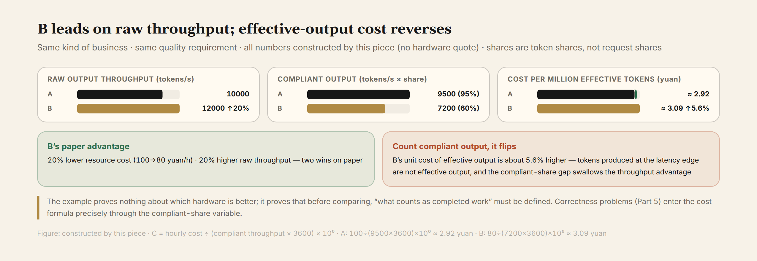
Now the arithmetic. On the first two rows alone, B is cheaper with 20% higher throughput. Add the third row: effective outputs are Q_A = 9,500 Token/s and Q_B = 7,200 Token/s. Running cost per million effective tokens:

C_A = 100 ÷ (9,500 × 3,600) × 10⁶ ≈ 2.92 yuan
C_B = 80 ÷ (7,200 × 3,600) × 10⁶ ≈ 3.09 yuan

The conclusion reverses: B’s resources cost 20% less, raw throughput is 20% higher, yet per-unit running cost on effective output is about 5.6% higher.

The example proves nothing about which hardware is better; the numbers are constructed. What it proves: before comparing, you must define what output counts as completing the task. The correctness question of Part 5 enters the cost formula directly through the “compliant share” variable.

The break-even line. The example pushes one step further. Holding A’s cost and compliant share fixed, B matches A’s unit cost when its effective output reaches 80 × 9,500 ÷ 100 = 7,600 Token/s, which is about 63.3% of its 12,000 Token/s raw throughput. So 63.3% is this example’s break-even line:

Reaching exactly 63.3% is only parity; above it, B gains the per-unit running-cost advantage.
The line compares running costs only, excluding one-time investment.
It moves with the two options’ cost ratio and throughput ratio; new quotations demand recomputation.

Figure 1 The cost-reversal example: B leads on raw throughput and resource cost, A overtakes on effective output, at 2.92 versus 3.09 yuan per million effective tokens (constructed)

4. From Single Points to Load Curves

The example used single points; the real object of comparison is a load curve. “Load” itself must first be defined through tool parameters. The relevant vLLM semantics:

--request-rate: a finite value means controlled arrival load, Poisson by default; inf means full-concurrency stress. The two measure different things; capacity questions take the finite rate.
--burstiness: effective only under finite rates, tuning arrival volatility with a Gamma distribution. 1.0 is plain Poisson; lower is burstier; higher is more uniform.

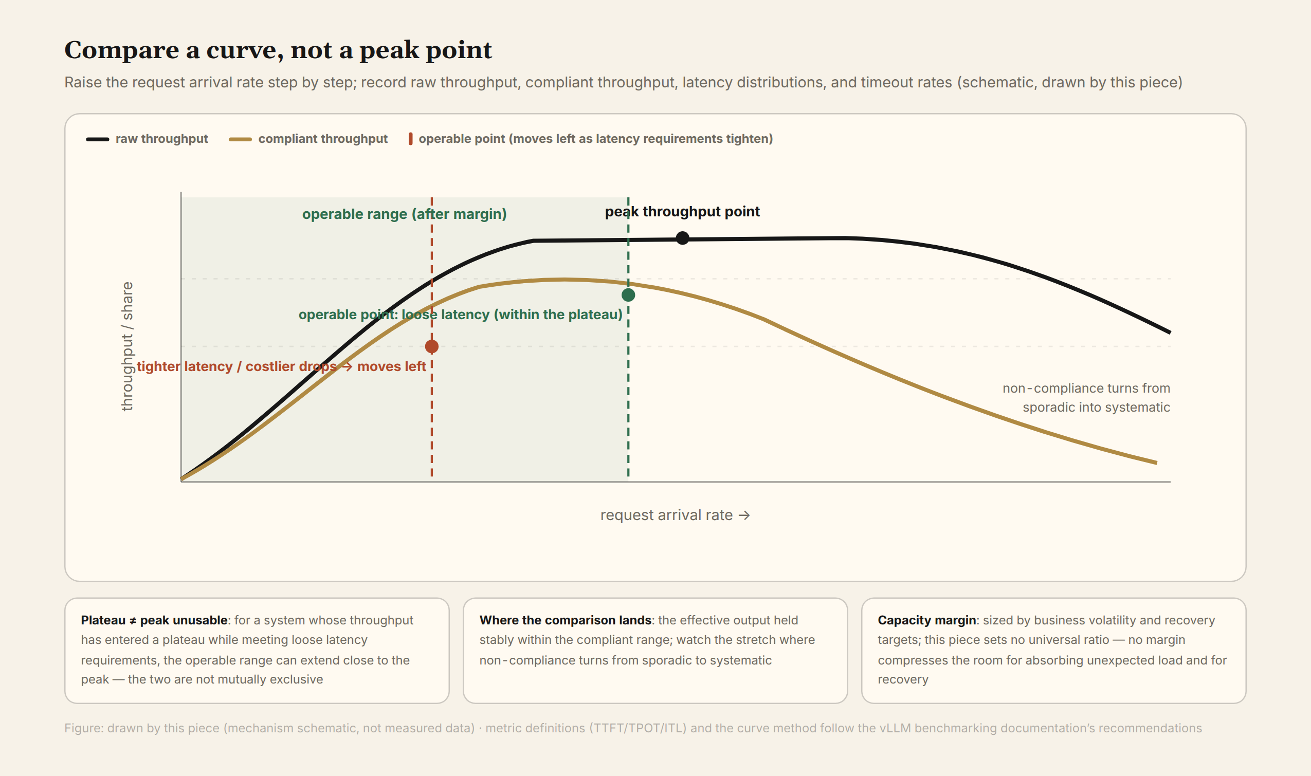
How to draw the curve. Raise the arrival rate step by step; at each tier record raw throughput, compliant throughput, TTFT and generation-latency distributions, and timeout and failure ratios. Watch the segment where non-compliance turns from sporadic events into systematic ones. What deserves comparison is the effective output stably sustained within the compliant range.

Do not miss client-side queuing. --max-concurrency caps the client’s in-flight requests to simulate backpressure, but it also moves queuing to the client: a request first waits for a concurrency slot, and after being sent the server may respond quickly. Looking only at post-send TTFT misses that wait. The documentation provides two metrics for this:

client_queue_time: time spent waiting for the client’s concurrency slot;
e2el_including_client_queue: under finite rates, the end-to-end duration counted from the moment the request should have started under the arrival plan, including client queuing.

Put both into the comparison table. Otherwise two options’ “similar TTFT” may only mean one hides its waiting on the client. This is a note on measurement semantics, not a measured conclusion about any specific system.

Where the operating point sits is a business decision, not an engineering default. If throughput has entered its plateau and latency requirements are loose, the operable range can extend toward peak; as latency tightens or the cost of drops rises, the operating point moves forward. Headroom follows business volatility and recovery objectives, with no universal ratio. Leaving no headroom squeezes the room for absorbing bursts and recovering from failures. Volatility can be absorbed by capacity or traded against with short queuing, but both have limits.

Figure 2 Load curves and the operable range: throughput plateaus, compliant throughput varies with load; as latency requirements tighten, the operating point moves forward (illustrative)

5. Preconditions for Comparability: Consistency and Caching

Two consistencies must hold when comparing curves:

Workload consistency: the same request set, the same order and prefix distribution, the same cache policy (both from a clean start, or both warmed to their steady states). Both sides being “cold-started” does not automatically mean comparable, since public-prefix hits can occur inside a single run. What is controlled is these variables themselves, not a one-line label of “cold start” or “warm cache.”
Consistency of metric definitions and timing windows: numbers from cold and warm caches, or from different precision configurations, do not go into one table.

Caching deserves separate treatment. The vLLM documentation warns that repeated benchmarks against the same server may reuse prefix cache and inflate measured throughput. The right move is not to disable caching wholesale but to evaluate twice:

Controlled comparison: both sides under identical cache conditions, isolating the implementation difference;
Business replay: keeping the real repeated-prefix distribution, assessing the cache’s actual business benefit.

A system serving mostly repeated document QA and one whose prompts almost never repeat should not share a cache-hit assumption. Using the former’s throughput to argue the latter’s procurement books someone else’s prefix-reuse gains as your own.

6. Beyond Running Costs: One-time Investment and Recurring Maintenance

Half the economic ledger is often missed: the spending that never appears on the hourly bill. It comes in two classes:

One-time investment: first-migration adaptation (layout conversion, pipeline rearrangement, interface hookup) and first acceptance (the workload of Part 5’s verification path).
Recurring maintenance: combination regression after version upgrades (Part 7), daily operations, and failure losses. These enter the period’s total cost or net savings as they occur; they are neither double-counted with one-time investment nor treated as pay-once-and-done.

The payback formula.

Payback period = one-time investment ÷ net savings per period
Net savings per period = the two options’ running-cost difference − the difference in their extra maintenance costs (amortized to the period)

The preconditions: equal task volume, equal compliance requirements, comparable time windows. Costs already counted in running costs are not deducted again from the maintenance difference. Net savings must be positive: if the new option’s net savings under these conditions is zero or negative, for instance higher running cost with lower effective output, it cannot recover the one-time investment. This piece gives the frame and fills in no numbers; substitute real quotations and loads, and the conclusion comes out by itself.

Which cost line each part’s technical choices land on:

Part 2’s layout conversion: on per-layer activations, it enters every request’s running time;
Part 3’s padding and overlap quality: decides how much effective throughput the same bandwidth yields;
Part 4’s supply line, the path moving KV data from device memory into the Cube core: decides attention latency and reachable batch sizes;
Part 5’s verification path: a one-time investment that also shapes running cost through the compliant share;
Part 7’s version upgrades: each demands a fresh round of regression testing.

Conclusion

This comparison method points at no particular hardware’s superiority; it changes which questions to ask:

kernel throughput varies with shape;
service capacity must be measured end to end under given conditions;
procurement compares the running cost per unit of effective output under a given load and compliance requirement, and whether and how quickly the one-time investment is recovered.

Part 7, the final part of the series, raises the view one more level: how to judge whether the ecosystem this wave of open source is building is truly accumulating, or merely releasing.

Sources and computation notes: This piece is based on vLLM public documentation, the DeepGEMM README, and this piece’s constructed examples, fact-checked as of October 7, 2026.

The definitions of TTFT, TPOT, and ITL; the prefix-cache warning; the “metric terminology is not standardized; compare measurement points and formulas” note; and the semantics of --request-rate, --burstiness, --max-concurrency, client_queue_time, and e2el_including_client_queue (including its schedule-relative meaning) come from the vLLM benchmark documentation (stable page; the document itself carries no version number, and the field names follow that version).
MegaMoE’s two data points under one configuration (96 experts, hidden 7168; tokens 64 → 256; throughput 266.4 → 659.2 TFLOPS) come from the DeepGEMM README, official results; the table does not mark a precision configuration, and no extrapolation to other shapes is implied.
Section 3’s example and break-even derivation (100 vs 80 yuan; 10,000 vs 12,000 Token/s; 95% vs 60%; 2.92 vs 3.09 yuan; about 5.6%; about 63.3%; about 7,600 Token/s) are this piece’s constructed data and algebra, corresponding to no hardware quotation.
The definition of compliant tokens, the split between one-time and recurring investment, and the payback frame are this piece’s judgment framework. No specific payback numbers are given.

No hardware measurements were made. This is Part 6 of the DeepSeek Ascend open-source series.