
A 10,000-GPU cluster: how many sandbox servers should sit beside it?
The card count alone does not answer it. The same round of training, given seven days or fourteen, changes how much training data must be delivered each second; how much inference compute it needs, and how many task environments it occupies, change with it. The training ground here means the sandbox infrastructure that hosts agent tool execution and task state: it receives the model’s actions, executes the task, and returns results; it does not generate model output.
Fix the task first: 1,000 outer iterations within one week, each consuming 4,096 trajectories. That is about 4.1 million in all, an average of 6.8 per second. This is the number that finally enters training batches; trajectories generated but filtered or discarded are not yet counted.
From this demand, this piece computes the inference-side throughput threshold and the environment-side average occupancy, then checks whether training updates can keep up.
1. A One-Week Target: 6.8 Effective Trajectories per Second
Infrastructure failures, timeouts, stale versions, or recipe filters all consume generation capacity. Write p for the effective intake rate; raw generation demand is effective-trajectory demand divided by p.
What is counted here is whether a trajectory enters a batch, not whether the task succeeded: failed trajectories can still be valuable training samples. The measurement should hold the task mix and batching requirements unchanged; it cannot be raised by preferentially consuming short trajectories.
The table below lists this piece’s settings together with observed references cited from the paper:
| Parameter | Value | Source |
|---|---|---|
| Outer iterations | 1,000 | this piece’s assumption |
| Trajectories consumed per iteration | 4,096 (512 tasks × 8 samples, GRPO group comparison) | this piece’s assumption |
| Time constraint | 7 days (604,800 s) | this piece’s assumption |
| Output per trajectory | about 33,000 tokens (64 interaction steps × 512 new tokens each; an interaction step is one model action plus its environment feedback) | this piece’s assumption |
| Card split | 7,000 training, 3,000 inference | this piece’s assumption |
| Per-card output throughput scan points | 60, 75, 200 tokens/s/card | this piece’s assumption |
| Trajectory environment duration | 1,044 s (paper’s container median lifetime of 17.4 minutes used as the mean) | paper (DSec, arXiv 2609.22978); substitution is this piece’s assumption |
| Per-node density | containers 3,200 / microVMs 800 (demonstrated operating points); sample-day peaks 1,048 / 524 | paper |
| Platform creations per day / peak online | about 3 million / over 380,000 | paper |
| Production unit and cloud spillover | 160 nodes; above 80% utilization offload to cloud, 200 cloud VMs absorbing about 30% of peak overflow | paper |
Scope and boundaries: 60, 75, and 200 are scenario scan points, not measurements; DSec’s figures serve only as references for the environment side’s scale and behavior, not for inferring DeepSeek’s actual GPU ratio; what this piece computes is the time to finish the stated training budget, not whether 1,000 iterations reach a capability target; all boundaries follow from this piece’s assumptions and must be calibrated against measurements before deployment.
2. The First Threshold: About 74 tokens/s per Card
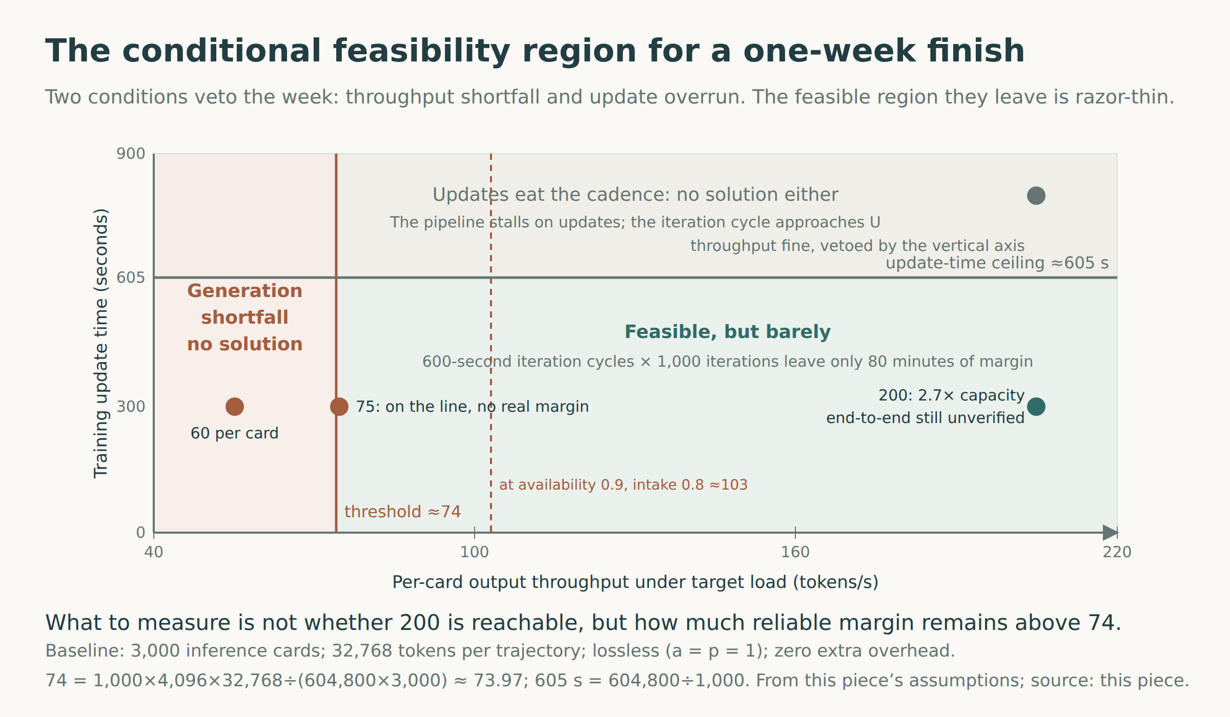
At 32,768 output tokens per trajectory, the total output for 4.1 million trajectories spread over one week and 3,000 inference cards gives a lossless threshold of about 74 tokens/s/card (1,000 × 4,096 × 32,768 ÷ (604,800 s × 3,000 cards) ≈ 73.97). 60 falls short, 75 leaves almost no margin, and 200 opens room to choose.
| Per-card output throughput (target load) | Equivalent trajectory capacity | Relative to 6.8/s | How to read it |
|---|---|---|---|
| 60 tokens/s | about 5.5/s | 0.81× | generation alone misses the deadline |
| 75 tokens/s | about 6.9/s | 1.01× | almost no margin for losses and overhead |
| 200 tokens/s | about 18.3/s | 2.7× | raw capacity is ample; end-to-end feasibility still unverified |
60, 75, and 200 are scenario scan points, chosen to watch the constraints below, near, and above the critical value. At the 200 tokens/s/card scan point, demand equals about 37% of the tier’s nominal capacity, a supply-demand ratio, not GPU utilization; where the bottleneck sits also shifts with the tier: at 60 it stays in generation, at 200 it moves to training updates and the environment side.
This threshold must be measured under the target Agent load. If the context, tool returns, or caching behavior change, the throughput must be re-measured.
How Throughput Is Counted
After an agent generates a stretch of actions, it waits for the environment to execute, then continues generating from the result; a single task may run through many such round trips (a rollout is the whole process of the model interacting with a real environment and generating training data). The same inference card yields different outputs in an online Q&A service than in agent training. This piece needs the latter: output throughput under target load, the output tokens each card produces while the inference service runs under the target context, tool returns, and caching conditions, before subtracting trajectories that never enter a batch. A single trajectory’s completion time is also bounded by environment execution and feedback latency, and cannot be derived from output token counts alone; this piece averages throughput over the deadline.
This piece measures inference output in output tokens; the cost of input processing, tool returns, and caching behavior shows up in the measured throughput under target load. Even with prefix KV reuse, output token volume is not the whole compute cost. In measurement, divide the inference pool’s total output by the GPU card-seconds allocated over the measurement window; do not count only devices that are actively decoding, or use kernel execution time as the denominator.
Counting losses raises the threshold accordingly. Write a for the availability of generation-service time and p for the effective intake rate, the two losses entering running time and samples respectively: with a = 90% and p = 80%, and assuming the average output across all attempts stays at 33,000 tokens, 73.97 ÷ (0.9 × 0.8) ≈ 103 tokens/s/card. If a measurement already includes one of these losses, do not discount it again; substituting an online Q&A service’s throughput for rollout throughput means the numerator and the denominator are not measuring the same thing.
3. An Average of 7,100 In-Flight Environments
Under the baseline assumptions: one environment per trajectory, an average occupancy of 1,044 seconds, and every trajectory entering a batch. By Little’s law, average in-flight count equals arrival rate times average occupancy: about 6.8 per second corresponds to about 7,100 in-flight environments.
With intake losses counted, the number scales by 1/p only if the average environment occupancy across all attempts stays unchanged. A task that exits immediately at initialization failure and one discarded after running long consume different amounts of environment; both need to be measured together.
One systematic understatement deserves note: Little’s law wants the average occupancy, while the 1,044 seconds substituted here is the median lifetime, and the distribution is strongly right-skewed (the container p99 in Section 4 is about 13 times the median), so the mean likely sits well above the median. Roughly fitting a lognormal to the container-side p50 and p99 gives an average occupancy of about 1,900 seconds and an average in-flight count of about 13,000, close to twice the baseline; that is a directional estimate, and the actual factor depends on the true distribution. A one-line consistency check between the two settings: 33,000 tokens of output ÷ 1,044 seconds of occupancy ≈ a single-stream decode speed of 31 tokens/s (about 17 tokens/s at the 1,900-second mean), before subtracting tool-execution time, so trajectory length and environment duration are broadly compatible.
After computing 7,100 average in-flight environments, one datum is still missing before a node count: how many environments one server can hold at the target latency when running this class of tasks.
DSec gives per-backend operating densities: 3,200 containers per node as a demonstrated operating point and 800 microVMs, with the paper’s own words that these are demonstrated operating points, not hard limits; the sample-day per-node peaks were 1,048 containers plus 524 microVMs, each backend its own peak, and adding them assumes both peak at the same moment. Here three terms need distinguishing:
- Observed density: how many environments this server has held at some point.
- Service capacity: how many it holds while meeting latency and reliability requirements.
- Planning capacity: what one commits after faults, bursts, and fragmentation.
The paper’s numbers are mostly the first kind; a configuration commitment needs the third, and observed density cannot serve directly as another system’s capacity commitment.
Before dividing, align the units. 160 nodes, 30,000 cores, 250TB: about 188 cores and 1.56TB per node on average; node specs are not uniform, and comparing node counts must state cores, memory, and service capability together.
Back to the opening question. At the sample-day observed per-node container peak of 1,048, the 7,100 in-flight environments need about 7 servers; at the mean-corrected 13,000, about 13. At the demonstrated operating point of 3,200, only 3 to 5. Those 13 are an arithmetic floor: counting an 80% intake rate puts the in-flight count at about 16,100 and the need at about 16 servers; at the 500-second cadence, which raises the effective supply to 8.19 trajectories per second, the raw generation rate is about 10.2 per second, in-flight about 19,500 and the need about 19 servers. I would plan for around 25 servers, leaving room for faults, bursts, and the gap between observed density and service capacity. Against one of DSec’s 160-node production units, that is about one-sixth the size; the reason is that this piece counts only the steady state of a single training run, without evaluation, environment building, or multiple teams sharing the platform.
Average concurrency only describes steady state. Sizing the environment side means answering three questions separately: whether in-flight capacity (memory, storage, instance quotas) suffices; whether tool-execution latency, mean and tail, and result-verification throughput meet requirements at the target concurrency; and how long a batch of simultaneously launched environments takes before its first effective interaction. A more robust accounting unit for environment consumption is sandbox-seconds, CPU core-seconds, and memory GB-seconds accumulated per trajectory attempt: one trajectory can span multiple sandboxes (rebuilt midway) or keep state after ending; evaluation and environment-building loads add on top.
4. Cadence, Margin, and Consistency
Enough inference capacity does not by itself mean training finishes on time. How much generation and parameter updates can overlap is the next question.
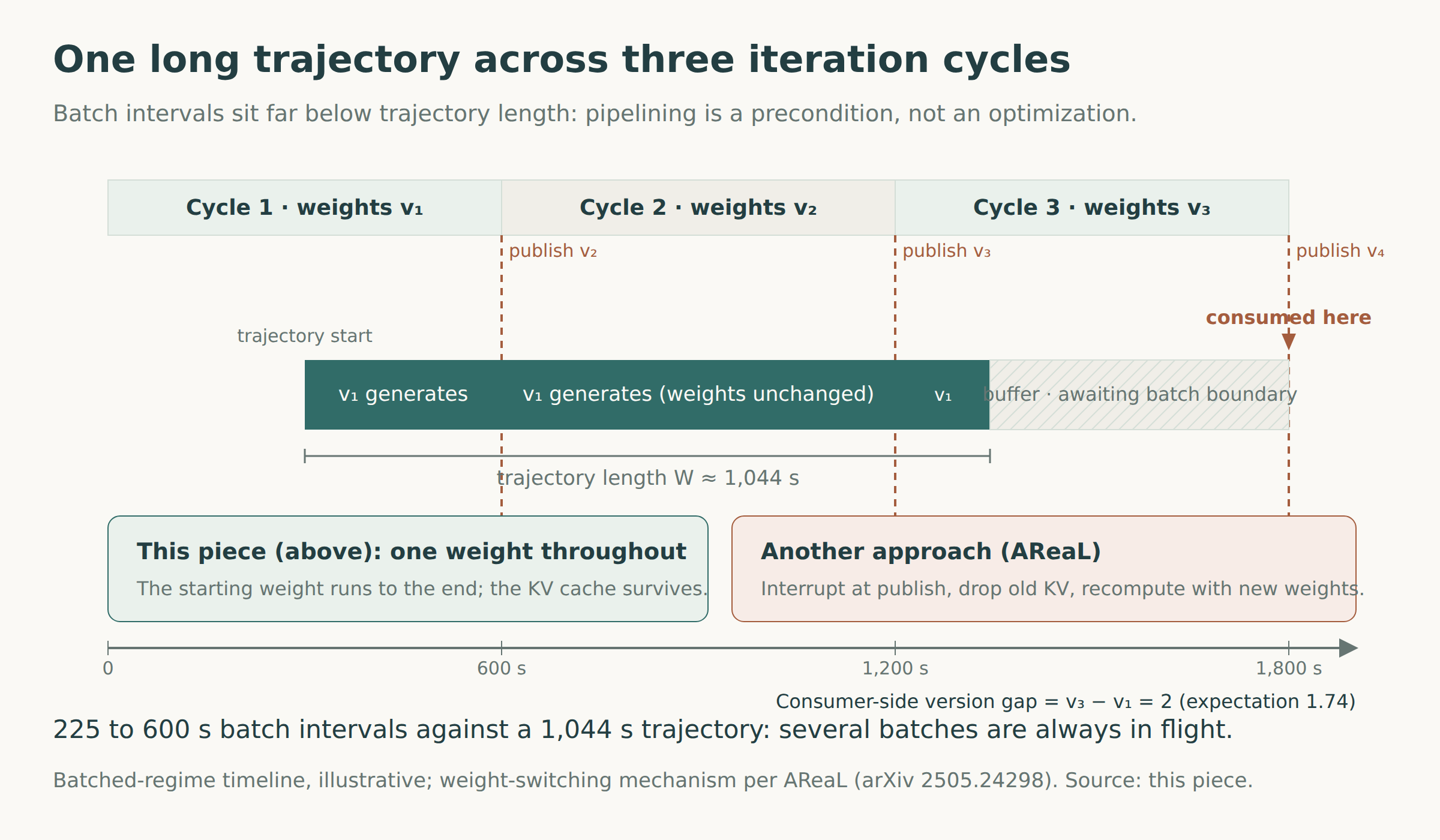
This piece assumes asynchronous generation and batched training. At the end of each iteration cycle (the interval between adjacent outer iterations), one weight version is published, and a single trajectory runs on one version of the weights from start to finish. An outer iteration consumes a batch of trajectories and completes a training update, possibly containing several optimizer updates; a weight publish means a new version becoming visible to the inference side.
In a steady pipeline, the interval between full batches can be shorter than a single trajectory’s running time. What makes this work is several batches in flight at once: one batch is completing while the next has been running for a while. This gives the training side a continuous supply of data, and leaves trajectories of different weight versions in the system at the same time. A shorter cadence raises pressure in two places: training updates must keep up, and weight switching must handle the trajectories still running and their KV caches. How long an update takes, whether a trajectory may switch weights mid-run, and how much cache must be recomputed after a switch together change the effective capacity; capacity cannot be planned on ideal throughput first, leaving consistency problems to the deployment stage.
Write the cadence as a checkable condition. Let B be the number of trajectories consumed per batch, R_eff the effective supply rate that meets the mixture and freshness requirements, U the training update time per outer iteration, and n the iteration count. Under the ideal approximation of fully overlapping generation and updates, the steady-state iteration cycle:
L ≈ max(B / R_eff, U)
Completing the full run additionally requires:
T ≈ n × L + T_extra ≤ T_budget
T_extra collects startup, teardown, and non-overlappable overheads not counted elsewhere; T_budget is the time budget. This extra overhead must be kept distinct from the stall losses already counted in throughput measurement, to avoid double counting.
U is another variable that must be measured; it depends on the training card count, batch size, parallelism strategy, and optimizer updates per iteration cycle, and this piece has no measurement of it. Take the 60 tokens/s/card scenario: the weekly output demand is about 222,000 tokens/s and the inference side is short about 700 cards; moving about 700 cards from training covers that generation gap, and the training side drops to about 6,300 cards, stretching update time by about 11% if it scales inversely with card count. The real allocation can only move in units of model replicas and parallelism groups.
The Spare Inference Capacity: Fewer Cards, or a Shorter Schedule?
Assume generation and updates overlap fully: 600-second cycles over 1,000 iterations take 600,000 seconds. The week has 80 minutes left for startup, teardown, and other extra overhead, which is not much room; 600 seconds is only a boundary point; any extra overhead pushes past one week.
Shorten the cycle to 500 seconds and the picture changes. After the main loop, the nominal time margin rises to about 17.3%. That margin can absorb retries, stalls, and load fluctuation, but it demands a higher supply rate: 8.19 effective trajectories per second entering training, about 21% above baseline.
Keeping the lossless and fixed-trajectory-length assumptions, the inference-side threshold rises to about 89.5 tokens/s/card. If average environment occupancy also stays unchanged, in-flight environments rise from about 7,100 to about 8,550 (about 15,600 under the mean estimate). Time is roomier; the demands on both inference and environment have risen.
Weight publishing still has to be checked. If weights are still published once per cycle, new versions appear faster, and long trajectories that have not finished may cross more versions. The system must decide whether to keep the old version and let tasks finish, or switch weights and absorb the cache and sample consequences.
So once the inference side has slack, the question is not only how many fewer cards it can run on. Compare whether spending the slack on a shorter schedule beats spending it on lower cost; the answer depends on whether update time, long-tail load, and sample freshness can take a faster cadence.
Consistency: What Happens to Old Trajectories When Weights Change
I lean toward letting old trajectories finish on their old weights, with each group of 8 trajectories starting on one version, and keeping the most recent 10 versions; on overrun the whole group is handled together (dropped entirely, or down-weighted), never mixing versions within a group. The reason comes from this piece’s own recipe: GRPO compares 8 samples within each group, and samples within a group should come from one version of the policy. Under this piece’s lifetime fit, a cap of 4 would push about one-fifth of trajectories over the limit at the 600-second cadence, close to the entire p = 80% loss budget in Section 2; a cap of 10 brings it to about 5%, or about 7% at the 500-second cadence. All of these are per-trajectory rates; under whole-group dropping it is the longest trajectory in a group that decides, and the group-level rate sits between 5% and about 35% (7% to about 46% at the 500-second cadence), depending on how strongly durations correlate within a group. Computed per group, a cap of 4 at the 600-second cadence carries an upper bound of about 83% (1 − 0.8⁸). With a cap of 10, at the group-level upper bound, dropping groups already exceeds the p = 80% budget, and the remaining options are whole-group down-weighting or a higher cap. The tolerable version gap has no measurement basis yet, so 10 is provisional; it firms up with the measurements Appendix A1 lists. AReaL (arXiv 2505.24298) chose the other way: on a weight-update request it interrupts all in-flight generation, drops the KV caches computed under the old weights, recomputes with the new weights, and continues generating. That trade solves the scheduling problem at the cost of recomputation and of the “switched mid-trajectory” definitional question. AReaL applies separate PPO handling to stale data and mixed behavioral policies; this piece borrows only the engineering practice, and whether it transfers to a GRPO recipe still needs separate verification. By contrast, keeping 10 versions resident means multiple weight versions live at once: it occupies inference memory, dilutes batching, and throughput should also be measured with the target number of versions resident.
Freshness: Mean Version Gap, Tail, Exceedance Rate
The version gap is the number of weight versions a trajectory crosses from start to consumption. Under this piece’s idealized timing, a 600-second iteration cycle corresponds to a mean version gap of about 1.7 by the median lifetime, or about 3.2 under the mean estimate (derivation in Appendix A1); under either convention, the tail deserves the closer look: taking sandbox lifetime as a proxy for trajectory duration, the cited container and microVM p99 lifetimes are about 13,900 and 12,800 seconds (about 3.9 and 3.6 hours, read from the distribution in the paper’s Figure 7; the paper’s text gives only a lower bound of over three hours), corresponding to about 23 and 21 publish cycles under the 600-second cycle; actual version gaps also depend on the starting version, queueing, and consumption timing. Runtime should therefore record the mean and tail version gaps and the group-level exceedance rate together; see Appendix A1 for how the cycle, version gap, and stability relate.
Sidebar: Same Week, Why Some Training Runs 30 Steps
Xiaomi’s MiMo-V2.6 reinforcement-learning run (official release article; released September 22, 2026, trained in under six days by the official account) has a set of official numbers: the Flash and Pro runs each completed 30 RL steps over roughly 750,000 trajectories (the official wording does not make clear whether the count is per model), 1,568 samples per update, fully asynchronous architecture, context up to 1 million tokens, and 3.5 to 3.7 billion tokens per step.
Why does a similar week hold only 30 steps for another run? The official numbers answer it directly: roughly 750,000 trajectories ÷ 30 steps ≈ 25,000 trajectories per step, while a single update consumes 1,568 samples, so each RL step packs about 16 optimizer updates. MiMo’s “step” is equivalent to several of this piece’s outer iterations. At 3.5 to 3.7 billion tokens per step ÷ 25,000 trajectories, each trajectory runs about 140,000 to 150,000 tokens; that conversion counts every token as rollout generation, is unconfirmed and is not used to adjust parameters for now. Before comparing resource demands, the accounting of iterations, samples, and tokens must be aligned.
5. Handling the Peak: DSec’s Cloud Spillover
DSec uses cloud VMs to absorb transient sandbox peaks while steady load stays local; when local utilization passes 80%, the placement engine routes eligible new requests to the cloud, and in production one scale unit of 200 cloud VMs absorbed about 30% of peak overflow. Production sizing therefore decides which loads stay local and which can spill elastically, and requires the image distribution, state, and scheduling paths to support that split. DSec moves its container runtime and EROFS image-loading path onto cloud VMs unchanged, with image sets synced offline to cloud storage.
DSec discloses the mechanism that absorbs part of the peak overflow, but that share cannot directly split the 380,000 peak-online figure. Back-computing capacity first requires aligning what is counted: whether online counts include cloud, whether spillover counts requests or concurrency, and which tasks are eligible for routing. For deployment, first draw the lines: which stretch of the load the local base, elastic capacity, and queueing limits each take. Peak online counts serve as a cross-check, not as something to divide back into server counts.
Ending: What to Measure, and How It Changes Decisions
Before deployment, four things need testing:
| Quantity to measure | Suggested measurement | What it decides |
|---|---|---|
| Effective-trajectory supply and consumption | under a fixed task mix, record separately the supply rate of trajectories meeting intake conditions and the rate at which training actually consumes them | whether generation meets the candidate cadence, training consumes in time, and the full budget completes on schedule |
| Training update cycle | separate data wait, update service time, publish and non-overlappable overhead | whether the 7:3 split holds; whether a 600-second iteration cycle is workable |
| Environment service capability | online count, provisioning latency, tool-execution latency under the target task mix | in-flight capacity and safe density |
| Freshness and cache recomputation | mean and tail version gaps, group-level exceedance rate, the correlation of durations within a group, cache recomputation after weight switches | whether pipelining keeps delivering effective capacity |
Testing should run in one end-to-end configuration and task mix, observing trajectory supply, training consumption, environment latency, and version gaps together, across steady state, bursts, and the long tail. Only when these requirements hold simultaneously do the calculations above translate into a configuration.
If only one thing can be tested first, test single-card rollout throughput under the target Agent load. It decides whether the deployment lands at the 60 tier or the 200 tier, and whether the bottleneck sits on the generation side or the training side.
Appendix
A1 Discrete Derivation of the Version Gap
Timeline: weights publish in batches, once per iteration cycle; a trajectory starts at a random point within a cycle window and runs on one weight from start to finish (no mid-run switch), then enters a buffer and is consumed at the next batch boundary. Write W for the trajectory duration and L for the iteration cycle; under batched publishing the weights change version every L seconds, and the version gap is the number of versions a trajectory crosses from start to consumption. Under the consumer-side convention, the version gap equals the current version at consumption minus the current version at start (new weights publish only after consumption), and its expectation is exactly W divided by L. One waiting term is easy to overcount: in seconds, a buffered sample waits half an iteration cycle on average; in version counting, the wait ends at the consumption boundary and contributes zero versions, so no extra half is added (discrete-timeline model, uniform start times as a steady-state idealization). Under the post-publish convention, every sample adds a constant 1. The whole derivation belongs to an idealized model with a fixed publish order, uniformly distributed starting phases, no extra backlog, and consumption at the next boundary after completion. It serves only as a comparison baseline; actual version gaps may sit above or below it.
Substituting numbers (W = 1,044 s): at a 600-second cycle the expectation is about 1.7 (probability about one-quarter that the gap is 1, three-quarters that it is 2); about 4.7 at 224 seconds; about 1.4 at 746 seconds. At the 1,900-second mean, the three tiers give roughly 3.2, 8.5, and 2.5. The 224 and 746 seconds come from the batching intervals of 4,096 trajectories at the 200 and 60 tiers (4,096 × 32,768 ÷ (3,000 × throughput)). Under this setting, the longer the cycle, the smaller the version gap, because publishing locks to batches; a tolerable mean version gap converts into a lower bound on the cycle, while the data’s wall-clock age grows with it. Under mechanisms that decouple publishing from training iterations (common for long-tail loads), the version gap grows with residence time times publish frequency and is managed by task grouping or replay. The theoretical reference is the asynchronous-GRPO stability analysis (arXiv 2607.01083): the stability boundary is characterized approximately by the product of the synchronization interval S and the learning rate η, with the maximum stable learning rate shrinking roughly as 1/S; the O(Sη) bound on the update bias introduced by staleness relies on local regularity conditions. That paper defines the synchronization interval S in optimizer updates, while this piece counts published versions in outer iterations; the two conventions do not transfer, and this piece draws no algorithmic-stability guarantee from it. To give a quantitative freshness boundary, the missing measurements are the weight-publish period, the learning rate’s stability region, and the maximum tolerable version gap.
A2 Remote Sensitivity
What follows are single-factor scenario calculations: average trajectory duration and environment density are held fixed. In a real speedup both may change, so these results are for observing parameter effects, not capacity forecasts. Holding only this piece’s average occupancy time fixed, 3,000 inference cards at 1,000 and 2,000 tokens/s/card correspond to about 96,000 and 191,000 average in-flight environments respectively (roughly 174,000 and 348,000 under the 1,900-second mean). Continuing to apply the two container-side historical densities: the sample-day peak of 1,048 gives about 91/182 nodes and the demonstrated operating point of 3,200 gives about 30/60 arithmetically equivalent nodes (roughly 166/332 and 54/109 under the mean; the two microVM densities are unused). These numbers show only how the density assumption moves the conversion, not committable capacity under a sped-up workload, and actual node counts still require re-validated service capability under that load. Note this already leaves the one-week-target scenario: the demand rate rides capacity, in-flight counts and nodes scale up proportionally, and these numbers must not be used to answer “how much to provision to finish in a week.”
Relaxing the constraint to two weeks means the raw generation-throughput constraint no longer excludes the 60 tokens/s/card scenario; updates, freshness, and the environment side still need verification. Under two weeks the iteration cycle can sit above 746 s, and under batched publishing the mean version gap drops slightly (about 1.7 to 1.4; roughly 3.2 to 2.5 under the mean estimate), but the cadence slows and the data’s wall-clock age grows.
These parameters govern different constraints: the training budget and deadline set the effective-trajectory requirement; output length, throughput, intake rate, and available time set the generation-side resources; environment occupancy and workload mix set average concurrency and service capacity; training update time and the publishing mechanism set the cadence the system can run. Which one deserves priority depends on the measured bottleneck and the parameter uncertainty under the target workload.
Sources and calculation notes: This article uses the public figures of “DeepSeek Elastic Compute (DSec): A Sandbox Infrastructure for Effective Agentic Training at Scale” (arXiv 2609.22978, submitted September 19, 2026) and design assumptions flagged by this piece; the cloud-spillover mechanism is from the paper’s §3.4, and per-node densities from its backend-specific demonstrated operating points and sample-day observations. Xiaomi MiMo-V2.6 figures come from the official release article and the public training dashboard, taken at official wording. Asynchronous-stability references: arXiv 2607.01083 (the Sη stability boundary of asynchronous GRPO); the weight-switching mechanism follows AReaL (arXiv 2505.24298), implementation details; the prefix-cache cost basis follows the Automatic Prefix Caching page of the vLLM stable documentation (docs.vllm.ai/en/stable/features/automatic_prefix_caching/). All deduction parameters are this piece’s settings, flagged where they appear. Data as of October 5, 2026.