
Two Paths: The Architectural Divergence of Kimi K3 and DeepSeek V4
In 2026, two of China's most technically deep AI teams delivered, within the same quarter, different answers to the question of "what comes after the Transformer."
In April, DeepSeek released V4: 1.6T total parameters, 49B activated, one-million-token context, KV Cache compressed to 10% of the previous generation. In July, Moonshot AI released K3: 2.8T total parameters, 104B activated, one-million-token context, 2.5x training efficiency improvement. Both models made it into the top tier on Arena blind tests. K3 briefly claimed the #1 spot on the Frontend Code Arena, while DSV4 had the highest weekly token usage globally.
But the technical paths they took to reach this position were almost entirely different.
Su Jianlin wrote an honest line in his K3 architecture article: "Linear+Full route vs Sparse route, which can go further is currently unknown." Behind this statement lies a genuinely open question: when the original Transformer attention cannot sustain million-token contexts, there are two paths forward, but no one knows which has the higher ceiling.
What did each path cost? Let's start with K3.
I. K3: Meticulous Calculation Under Constraints
K3's architecture formula: KDA + Gated MLA + Stable LatentMoE + AttnRes. Su Jianlin provided a complete public exposition of the logic behind each design choice. After reading it, the strongest impression: every K3 component is a trade-off made under specific constraints, choosing the least-bad option available under current conditions.
Attention: 69 Layers of "Compressed Memory" + 24 Layers of "Original Archives"
For million-token contexts, standard Attention is computationally infeasible. Even with MLA compressing KV, memory still grows linearly with sequence length. This constraint applies equally to all long-context models.
K3's solution: replace 69 of the 93 layers with KDA (linear recurrent attention). KDA does not retain KV for each historical token; instead, it continuously "writes" all history into a fixed-size recurrent state matrix S. For each incoming token, the matrix is updated in three steps: "forget → correct → write." No matter how long the sequence, the matrix size remains constant.
How large is each KDA layer's state matrix? K3 has 96 attention heads, each maintaining a d_head × d_head matrix. d_head = 128 (K3 technical report, Table 1, independent hyperparameter):
96 × 128² × 2 bytes = 3,145,728 bytes ≈ 3.0 MB/layer
69 layers total approximately 207 MB. Whether the context is 1K or 1M, this number does not change. This is K3's memory constant across 69 layers.
But linear recurrence carries an unavoidable cost: information loss. A fixed-size state is like a drawer that can only hold so many things — as new items keep coming in, old ones must be squeezed out. A function name defined 800K tokens ago may no longer be recoverable from linear memory. Yet precise content-addressable recall ("I remember seeing this word at that position") is precisely what code, long-document retrieval, and Agent tool calls demand.
So K3 retains 1 layer of Gated MLA (full attention) after every 3 KDA layers. These 24 MLA layers perform global token-to-token interactions, capable of precisely revisiting any historical position. Division of labor: KDA is "continuously updated working memory," MLA is "consulting the original archives."
The intellectual cost of this 3:1 ratio: 75% of layers perform lossy compression, only 25% can do precise retrieval. K3 compensates with the global attention of 24 MLA layers. Moreover, the final layer must be MLA, ensuring a global convergence before output. But for extremely fine-grained retrieval tasks (e.g., precisely locating a specific variable definition in an 800K-token codebase), are 24 MLA layers enough? The technical report does not provide ablation experiments on different KDA:MLA ratios.
The Conditionality of NoPE
K3's MLA layers do not use RoPE. This would be unworkable in a pure MLA model: removing RoPE from K2 noticeably degrades performance. Su Jianlin explains: KDA itself implicitly encodes positional information. DeltaNet's recurrent operations are non-commutative (doing A then B yields a different result from B then A), so ordering is inherently embedded in the computation. Combined with channel-wise decay providing recency preferences at different temporal scales, KDA replaces RoPE's functionality.
This is a classic constraint-driven choice: it's not that NoPE is better, but with KDA, NoPE becomes viable, saving the engineering hassle of tuning RoPE base or performing NTK interpolation when expanding the window from 256K to 1M.
Hardware Adaptation: Making the Algorithm Take the Shape GPUs Like
Su Jianlin's reason for modifying the KDA decay parameter lower bound is straightforward: if single-step retention approaches 0, the cumulative product's reciprocal overflows under BF16, forcing the use of inefficient special kernels. With the lower bound set at g_min = -5, each step's retention ≥ e⁻⁵ ≈ 0.0067, and the cumulative log-decay upper bound within a single 16×16 tile is -80 (16 × (-5)), so the reciprocal remains within BF16 range. Diagonal tiles can then use Tensor Core dense matrix multiplication.
This lower bound is unnecessary in theory, but BF16's dynamic range and Tensor Core's computation preferences force the algorithm to accept it. Su Jianlin's principle: an algorithm must run fast on GPUs to have value.
Stable LatentMoE: Taming Extremely Sparse MoE
896 routing experts select 16, plus 2 always-on shared experts, yielding a total activation rate of ~2.0%. Compared to DSV4's 256-select-8 (3.1%) and Mixtral's 8-select-2 (25%), K3's sparsity is the most extreme.
What extreme sparsity exposes first is numerical anomalies. SwiGLU's gate and up pathways produce unbounded activations that, when multiplied together, cause output variance to inflate dramatically. K3's countermeasure is SiTU: using softcap (β=4 for the gate + β=25 for the linear path) to cap outliers. GPT-OSS and DSV4 use Hard Clip here; Su Jianlin found that under identical bounds, softcap performs better — Hard clip has discontinuous gradients at the boundary, while softcap transitions more smoothly.
With numerical stability achieved, the scale problem surfaces next. LatentMoE first reduces dimensionality (7168→3584) for MoE then increases it (3584→7168), and the variance drift from 4-matrix chained multiplication is extremely hard to control. Ablation experiments pointed to a minimalist solution: add an RMS Norm before the dimension increase. Just this one addition stabilizes the chained multiplication scale, with an unexpected bonus of equivalent depth improvement.
With numerical and scale issues settled, the final adversary is routing imbalance. 896-select-16 means popular experts get selected repeatedly while unpopular ones waste parameters. QB (Quantile Balancing) uses a 1000-bin histogram to approximate global quantiles, leveraging distribution additivity for cross-machine aggregation with minimal communication. Testing showed no difference between 1000-bin and 10000-bin — precision is not the bottleneck; communication efficiency is.
II. DSV4: Same MLA, Different Direction
DSV4 also starts from MLA, but takes a completely different transformation route. It does not introduce linear attention; instead, it compresses attention across all layers.
CSA + HCA: Magnifying Glass and Telescope
DSV4's attention alternates between two compression strategies, each with a complete engineering implementation.
CSA (Compressed Sparse Attention) — a three-component system:
- KV Compressor: Every 4 tokens' KV is merged into 1 compressed entry via attention pooling (4:1). This is lossy compression — fine-grained information from 4 tokens is averaged into a single vector, but in exchange, KV Cache is reduced by 4x.
- Lightning Indexer: Compressed entries can still be numerous (~250K entries for 1M context after compression), so full scanning is infeasible. The Indexer uses a dual-encoder architecture for approximate nearest neighbor search, filtering top-k most relevant compressed entries for each query. Pro model k=1024, Flash model k=512.
- Sliding Window: Maintains uncompressed KV for the most recent 128 tokens. Language models depend heavily on recent context, where compressed entries suffer the most information loss; the Sliding Window preserves local precision.
HCA (Heavy Compressed Attention) is more aggressive: 128:1 compression ratio. 128 tokens are condensed into 1 entry at a very coarse granularity. But the number of compressed entries is small (~7,800 entries for 1M context), so queries can scan all entries directly without the Lightning Indexer. Also includes a Sliding Window of 128 for local precision.
The two alternate across layers. CSA performs precise localization (magnifying glass), HCA performs global perception (telescope), allowing the model to view context at different distance scales. Combined effect: at 1M context, KV Cache is only 10% of V3.2, and per-token FLOPs are only 27%.
Residual and Routing: mHC and Engineering Details
mHC (Manifold-constrained HyperConnection) expands the residual stream from 1 to 4 channels (hc_mult=4). Each layer dynamically mixes multiple residual streams via matrix B, giving information transfer multiple parallel channels. The original HC (proposed by the Kimi team) frequently suffered numerical instability; mHC adds manifold constraints to stabilize singular values near 1. Each layer applies mHC before and after attention/mlp: first compressing multiple streams into one for sublayer input, then distributing the output back across streams with dynamic mixing.
Compared to K3's AttnRes (which lets each layer actively choose which depth to read from), mHC is structural — all layers gain additional information channels but do not perform active selection. The former is more flexible; the latter is more stable.
Other engineering details: routing activation function changed from Sigmoid to Sqrt(Softplus(·)) (smoother gradients); early-layer dense FFN replaced with Hash-routinged MoE layers (reducing computational bottlenecks in early layers); DualPipe continued from V3 with scheduling adjustments for mHC; Muon optimizer replacing AdamW (borrowed from Kimi — both teams converged on the same optimizer choice).
The Intellectual Angle: What Each Path Lost
K3 and DSV4's attention transformations exact differently shaped costs on intelligence. Actual benchmarks can validate this theoretical judgment:
| Dimension | K3 | DSV4-Pro |
|---|---|---|
| FrontierSWE (Software Engineering) | 81.2 | ~70 |
| Program Bench | 77.8 | ~72 |
| Arena Frontend Code | #1 (1679 points) | #3 |
| Overall Capability Position | Global #3 (behind only Fable 5, GPT-5.6 Sol) | Close to Claude Opus 4.8 |
| Output Price (API) | ¥100/M tokens | ¥6/M tokens |
| Generation Speed | Slower (104B activated) | Faster (49B activated) |
Data sources: Arena.ai, Artificial Analysis, official pricing (2026-07).
K3 leads on complex programming tasks requiring precise long-range retrieval. FrontierSWE 81.2 exceeds GPT-5.6 Sol's 71.3, demonstrating that 24 MLA layers suffice for precise retrieval in programming scenarios. K3's #1 ranking on Frontend Code Arena is further bolstered by native multimodal capability enabling "vision in the loop" — writing code, checking screenshots, then revising — something the text-only DSV4 cannot do.
DSV4 is superior for cost-sensitive general-purpose scenarios. The precision loss from full-layer compression is acceptable in practice — performance approaches Opus 4.8, coding rivals GPT-5.6 Sol, but output price is only 1/16 of K3's. For everyday code assistants, Agent execution, and Chinese-language tasks that don't require extreme long-range retrieval, DSV4's "always semi-precise" approach is good enough.
The essential difference between the two costs: K3 preserves lossless global attention on 24 layers, at the cost of 75% of layers being lossy; DSV4 preserves the attention mechanism itself on all layers (only compressing the input), at the cost of all layers having degraded precision. The former is "mostly approximate, occasionally precise"; the latter is "always semi-precise." Which is better depends on the task's attention pattern: tasks needing occasional precise retrieval favor K3, while tasks needing continuous semi-precise global perception favor DSV4.
K3's cost: reduced frequency of precise retrieval. 75% of layers perform lossy compressed memory; only 25% can perform precise global token-to-token queries. For tasks requiring frequent retrieval of distant context (long codebase refactoring, multi-document cross-referencing), K3's 24 MLA layers are the only precise retrieval channel. Whether they suffice depends on the task's information density. If retrieval targets are sparsely distributed, 24 layers are enough; if many scattered details need simultaneous attention, they may fall short.
DSV4's cost: reduced attention resolution. All layers are compressed, meaning CSA's 4:1 and HCA's 128:1 ratios mean query tokens see compressed approximations rather than original KV. CSA's sparse selection relies on the indexer's predictions; when the indexer predicts poorly, relevant information gets missed. HCA's 128:1 compression is even more aggressive — distant fine-grained information gets averaged away during compression.
Which is better depends on the task's attention pattern: choose K3 for occasional precise retrieval, choose DSV4 for continuous semi-precise global perception.
Post-Training Headroom: Insights from DSV4 Flash 0731
DSV4 Flash 0731 provides a perfect natural experiment: same base model (284B/13B activated), architecture completely unchanged, only post-training redone. Results:
| Agent Benchmark | Flash Preview | Flash 0731 Release | Improvement |
|---|---|---|---|
| Terminal Bench 2.1 | ~70 | 82.7 | +18% |
| DeepSWE | 7.3 | 54.4 | +645% |
| Toolathlon Verified | 52.8 | 70.3 | +33% |
| Cybergym | 57.7 | 76.7 | +33% |
All 9 Agent benchmarks surpassed their own larger sibling V4-Pro Preview (1.6T/49B, 4x the body weight). This is the industry's strongest evidence for the thesis that "post-training matters more than pre-training."
From an architectural perspective, the two models have asymmetric post-training headroom.
DSV4 has larger post-training headroom for three reasons:
-
The precision loss from sparse compressed attention can be compensated by post-training. CSA's Lightning Indexer misses relevant information when predictions are inaccurate; HCA's 128:1 compression averages away distant details. Post-training can optimize the Indexer's routing strategy, enabling it to learn more precise selection for specific tasks. Flash 0731's DeepSWE jump from 7.3 to 54.4 is likely because post-training taught the Indexer to locate code-task-relevant entries more accurately.
-
The 49B-activation "underfit" base is easier to lift with post-training. DSV4 Pro has only 49B activations, doing less computation per token, meaning it may be "undertrained" during pre-training. Post-training (RL + SFT + multi-teacher distillation) can extract the base model's latent capabilities without increasing inference cost. K3's 104B activations perform more computation per token during pre-training, having "learned deeper," so post-training's marginal returns are relatively smaller.
-
K3's core limitation falls outside what post-training can address. K3's bottleneck is the information loss in 69 KDA layers — the forgetting in linear recurrent memory is architecturally inherent. K3 is already strong on programming tasks (FrontierSWE 81.2), indicating 24 MLA layers suffice for precise retrieval. But to improve further, the bottleneck becomes "not enough MLA layers" — an architectural problem, not a training one.
Where K3's post-training headroom lies: K3's technical report describes the post-training goal as "training a complete Agent loop" — three task domains × three reasoning effort levels, each with RL, plus multi-teacher online policy distillation and merging. Directions with remaining headroom include: better Agent tool-calling strategies, better long-horizon task planning (the K3 technical report demonstrated a 24-hour continuous GPU kernel optimization case), and vision-in-the-loop code iteration capability.
A testable prediction: If DSV4 Pro's release version receives the same magnitude of post-training upgrade, its Agent capability improvement will likely exceed what K3 would gain from equivalent post-training. Reason: DSV4's base is larger but activations are smaller, giving post-training a stronger "leverage effect" — a small amount of high-quality post-training data can unlock the untapped potential of a large-parameter base. K3's 104B activations have already "used" the base more fully, so post-training's marginal effect diminishes.
Su Jianlin's Observation: DSV4 Never Truly "Abandoned" MLA
DSV4 appears to have switched to a completely different attention mechanism, but Su Jianlin points out a detail most overlook: DSV4 uses head_dim=512, K=V-shared MQA, which is exactly MLA's decoding-equivalent form. DSV4 used MLA's equivalent form to ensure quality (Su Jianlin speculates), but training costs surged, prompting the introduction of Sparse and Compress to compensate.
The two routes converge. K3 replaces most layers with linear attention (Linear+Full hybrid); DSV4 compresses all layers with sparse compression (Sparse+Compress). Both start from MLA, both end at "KV Cache must be drastically compressed."
III. The Engineering Realization of Architectural Costs
At inference time, architectural divergence translates directly into a hardware procurement list.
KV Cache: The Fork in the Road
Let's examine the largest expense item: KV Cache. (The following assumes FP8 quantized deployment, with KV Cache computed in BF16.)
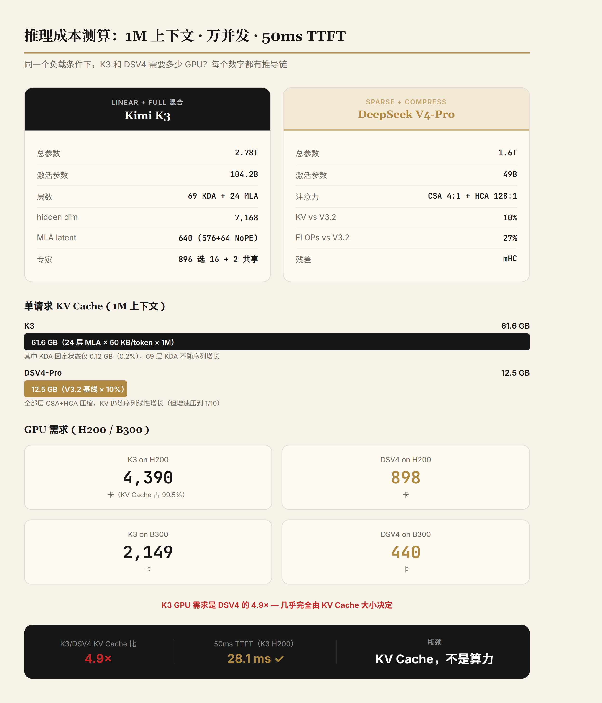
K3's 24 MLA layers: Per-token per-layer KV Cache = 640-dim latent × 2 (K/V dual latent, Gated MLA differs from standard MLA's single-latent design) × 2 bytes (BF16) = 2,560 bytes. 24 layers total 61.4 KB per token. 1M context single request: 61.4 GB.
Adding 69 KDA layers' fixed state of 207 MB, a single request totals approximately 61.6 GB. KDA's fixed contribution is 0.3% — 3/4 of layers are nearly "free"; the bottleneck is entirely on the 1/4 MLA layers.
DSV4's all compressed layers: V3.2 standard MLA is ~122 KB per token (61 layers × 2,048 bytes/layer). DeepSeek claims V4's KV Cache is compressed to 10% of V3.2, so V4 is ~12.2 KB per token. 1M context single request: 12.2 GB.
K3's per-request KV Cache is approximately 5x DSV4's. At 10K concurrency: K3 ~616 TB, DSV4 ~122 TB.
This 5x gap comes directly from architectural choices. K3 reduces the number of MLA layers (93→24) to save memory, but each MLA layer's latent dim is larger (640 vs 512), partially offsetting the reduction. DSV4 uses full-layer compression, achieving a higher effective compression ratio.
GPU Requirements: KV Cache Eats Everything
4,390 vs 877. This is the GPU count gap between K3 and DSV4 on H200 (141 GB) to support 10K-level concurrency. Breaking weights and KV Cache apart:
K3: Weights 2.8 TB (20 cards) + KV 616 TB (4,369 cards) ≈ 4,390 cards
DSV4: Weights 1.6 TB (12 cards) + KV 122 TB (865 cards) ≈ 877 cards
Weights account for only 0.5%~1.3% of total requirements. The 5.0x GPU gap (4,390/877) is almost entirely determined by KV Cache.
Deployment Architecture: Deriving Parallelism Strategies from Model Structure
The above numbers are "bare memory" estimates — assuming memory can be perfectly allocated. In actual deployment, each card must hold both weights and KV Cache simultaneously, and the trade-off between the two determines real concurrency capacity. The following references the SGLang team's public practice of deploying DeepSeek V3 on 96 H100s (LMSYS 2025-05), deriving parallel configurations from K3 and DSV4's architectural parameters.
Hardware basis: HGX H200 server, 8 × H200 SXM, single-card HBM3e 141 GB, bandwidth 4.8 TB/s, intra-node NVLink 4 aggregate bandwidth 900 GB/s, inter-node IB 400 Gb/s.
Step 1: Choosing Parallelism Strategy
Large model inference has three parallelism modes. Tensor Parallel (TP) splits intra-layer weights but requires all-reduce per layer, limited by the NVLink domain. Data Parallel Attention (DP Attention) lets each card independently process different request subsets, with KV Cache not replicated across cards. Expert Parallelism (EP) distributes MoE experts across cards.
How to choose? The key is the model structure.
Attention layers: Both models choose DP Attention. Reason: K3's 24 MLA layers' KV Cache is compressed to 640-dim latent (2,560 bytes/token/layer), and DSV4's all-layer CSA+HCA compresses to 12.2 KB/token. Both have small KV Cache, so DP Attention's per-card independent replication cost is acceptable. In contrast, TP provides little benefit for attention layers (matrices aren't large enough) while adding communication overhead.
MoE layers: Both models choose EP. This is the only feasible way to scale MoE across multiple nodes. The key question is EP scale.
Dense FFN: Both choose DP. K3 has 1 dense FFN layer, DSV4 has 3 (V4 replaced early layers with Hash-routinged MoE). TP causes severe fragmentation with large intermediate_dim, so DP is superior.
K3 unique: KDA layers require zero cross-card synchronization. When 69 KDA layers use DP Attention, each card maintains its own recurrent state matrix. State updates are purely local computations requiring no cross-card communication. This is a hidden deployment advantage of K3's architecture.
Step 2: Deriving EP Scale
The core constraint of EP: each card must fit its allocated expert weights and still have room for KV Cache. This requires first calculating per-expert size.
K3's 896 routing experts:
K3 total parameters 2.78T. Subtracting attention (~0.5T) and embedding (~0.1T), the MoE portion is ~2.2T. 896 routing + 2 shared = 898 experts:
Per routing expert ≈ 2.2T / 898 ≈ 2.45B × 1 byte (FP8) = 2.45 GB
Progressively testing EP scale until a single card can fit:
| EP Scale | Nodes | Experts/Card | Weights/Card | H200 Remaining | Feasible? |
|---|---|---|---|---|---|
| 8 | 1 | 112 | 274 GB | Insufficient | ❌ |
| 16 | 2 | 56 | 137 GB | 4 GB | ❌ (KV Cache space insufficient) |
| 32 | 4 | 28 | 69 GB | 67 GB | ✅ |
K3's LatentMoE dimensionality reduction (7168→3584) plays a role here: each token sends half-width 3584-dim data to 16 experts, halving routing communication volume. But with 896-select-16 routing at EP=32, each token on average sends data to 16/32 = 50% of nodes, so routing communication density remains high.
K3 minimum viable deployment: EP=32, 4 nodes 32 cards. Each card holds 69 GB weights, leaving 67 GB for KV Cache.
DSV4-Pro's 256 routing experts:
Per routing expert ≈ (1.6T - 0.3T) / 256 ≈ 5.1 GB (FP8)
| EP Scale | Nodes | Experts/Card | Weights/Card | H200 Remaining | Feasible? |
|---|---|---|---|---|---|
| 8 | 1 | 32 | 163 GB | Insufficient | ❌ |
| 16 | 2 | 16 | 82 GB | 56 GB | ✅ |
DSV4 can use EPLB (Expert Load Balancer) to expand 256 experts to 288 (adding 32 redundant replicas), allowing more flexible distribution. This is DeepSeek team's open-source solution, already implemented in SGLang.
DSV4 minimum viable deployment: EP=16, 2 nodes 16 cards. Each card holds 82 GB weights, leaving 56 GB for KV Cache.
Step 3: PD Disaggregation Design
Prefill (compute-intensive) and Decode (bandwidth-intensive) have completely different communication patterns and batch characteristics. SGLang's practice on DeepSeek V3 demonstrates that PD disaggregation can boost decode throughput by approximately 5x.
Core PD disaggregation mechanism: P nodes receive requests and execute prefill (large batch, Normal Dispatch mode to maximize throughput); after completion, KV Cache is transferred via RDMA to D nodes, which execute decode (small batch, Low-Latency Dispatch + CUDA Graph to minimize latency).
K3's PD disaggregation has one unique overhead: KDA recurrent state transfer. Standard Transformers only need to transfer KV Cache. K3 additionally needs to transfer 69 KDA layers' state matrices (207 MB/request). But 207 MB over an IB 400 Gb/s (50 GB/s) link takes approximately 4 ms, negligible relative to the multi-second to tens-of-seconds prefill phase.
KDA state behavior on D nodes differs from KV Cache — it's fixed-size and does not grow with sequence length. Per-request memory on D nodes:
207 MB (KDA fixed state) + 61.4 KB/token × current sequence length (MLA layer KV Cache)
At average context 500K tokens: 207 MB + 30.7 GB ≈ 30.9 GB/request. KDA state accounts for 0.7%.
DSV4's PD disaggregation is simpler: All layers use compressed KV Cache, at 500K average context 6.1 GB/request, RDMA transfer ~0.12 s.
Step 4: D Node Concurrency Capacity
D node concurrency capacity determines how many nodes are needed for 10K-level concurrency. Calculation: total memory available for KV Cache per deployment unit ÷ average per-request KV size = concurrent requests.
K3 on H200 (EP=32, 4 nodes/deployment unit):
Per-card KV Cache capacity = 141 - 69 (weights) - 5 (attention/embedding) = 67 GB
32-card deployment unit KV Cache total = 67 × 32 = 2,144 GB
Per-request average KV (500K context) = 30.9 GB
Concurrent requests/unit = 2,144 / 30.9 = 69 requests
10K concurrency requires 10,000 / 69 = 145 D deployment units × 4 nodes/unit = 580 D nodes
Plus P nodes (empirical ratio P:D = 1:2.5, per SGLang practice): 580 / 2.5 ≈ 232 P nodes
K3 on H200 total: ~812 nodes (6,496 cards)
DSV4 on H200 (EP=16, 2 nodes/deployment unit):
Per-card KV Cache capacity = 141 - 82 - 3 = 56 GB
16-card deployment unit = 56 × 16 = 896 GB
Per-request average KV = 6.1 GB
Concurrent/unit = 896 / 6.1 = 147 requests
10K concurrency = 10,000 / 147 = 68 D deployment units × 2 nodes/unit = 136 D nodes
P nodes: 136 / 2.5 ≈ 54
DSV4 on H200 total: ~190 nodes (1,520 cards)
| Deployment Dimension | K3 on H200 | DSV4 on H200 |
|---|---|---|
| EP Scale | 32 (4 nodes/unit) | 16 (2 nodes/unit) |
| Weights/Card | 69 GB (28 experts) | 82 GB (16 experts) |
| KV Cache Available/Card | 67 GB | 56 GB |
| Concurrent/D Unit | 69 requests | 147 requests |
| D Nodes (10K concurrency) | ~580 | ~136 |
| P Nodes (1:2.5) | ~232 | ~54 |
| Total Nodes | ~812 | ~190 |
| Total GPUs | ~6,496 | ~1,520 |
| Node Ratio | 4.3× | Baseline |
Compared to the earlier "bare memory" estimate of 5.0x, the actual deployment node ratio drops to 4.3x. This is because DSV4's per-card weights are larger (82 GB vs K3's 69 GB), leaving proportionally less for KV Cache, which narrows part of the gap.
Step 5: HiCache Offload Correction
The above derivation assumes all concurrent requests' KV Cache resides on GPU memory simultaneously. This is an upper-bound estimate. In actual deployment, not all requests are decoding at the same time.
Multi-level cache hierarchy. SGLang's HiCache organizes KV Cache into three tiers (from CSDN practical data):
- L1 (GPU memory): KV Cache for requests currently decoding
- L2 (CPU pinned memory): KV for recently-used requests not currently decoding
- L3 (SSD/distributed storage): KV for longer-idle or cross-instance shared requests
Requests only need KV Cache on GPU while decoding. After an API response is returned, if the user doesn't immediately send the next message (multi-turn), the KV Cache is offloaded to L2/L3. When the next request arrives, it's swapped back from L2/L3 to L1.
Agent scenario hit rate. The DualPath paper (Tsinghua + Peking University, with DeepSeek, 2026-02) notes that Agent workloads typically achieve KV Cache hit rates >95%. This means the vast majority of requests' KV can be served from cache without re-prefill. But it also means the system must manage a large volume of cached KV — whether on GPU, CPU, or SSD.
Deriving GPU residency ratio using Little's Law. The above derivation assumes all concurrent requests' KV Cache is simultaneously on GPU. In reality, not all requests are decoding at the same time — some are waiting for user input, waiting for tool returns, or in offloaded states. We can use Little's Law from queueing theory to precisely derive the actual residency ratio of KV Cache in GPU memory.
Little's Law: L = λ × W (average number of requests in the system = arrival rate × average sojourn time). Applied to inference services, the key variable is the total GPU time a request spends decoding vs its total sojourn time in the system:
GPU residency ratio ρ = W_decode / W_total
W_decode = total GPU time across all decode steps for a single request
W_total = W_decode + W_idle (idle time waiting for user/tool responses)
W_decode depends on output length and decode speed. Assuming average output of 1,000 tokens at a decode speed of approximately 200 tokens/s (per-request throughput at 10K concurrency):
W_decode = 1,000 / 200 = 5 seconds
W_idle depends on interaction patterns. Referencing the DualPath paper (Tsinghua + Peking University with DeepSeek, 2026-02, arXiv:2602.21548) Agent workload measurements — average 157 interaction rounds, 429 tokens appended per round — we can derive three scenarios:
| Scenario | W_decode | W_idle | ρ = W_decode/(W_decode+W_idle) |
|---|---|---|---|
| High-interaction Agent (continuous multi-turn, short intervals) | 5s | 5s | 50% |
| Standard API (user thinks for a few seconds before replying) | 5s | 15s | 25% |
| Low-frequency batch (scheduled tasks, long intervals) | 5s | 40s | 11% |
High-interaction Agents have short intervals (tool execution results return almost immediately), so GPU residency ratio approaches 50%. Standard API users think 10-20 seconds per turn, giving ρ ≈ 25%. Low-frequency batch processing spends most time waiting for scheduling, with ρ as low as 10%.
Taking the median of the three scenarios, ρ = 25%, as the standard estimate. This figure aligns with community practice data — Ant Group reported that enabling HiCache in general QA scenarios reduces GPU memory usage by approximately 78% (i.e., GPU bears only ~22% of KV Cache, consistent with ρ=25%).
Corrected D node counts (using ρ=25%):
| Deployment Plan | Upper-bound Estimate | ρ=25% Corrected | ρ=50% High-interaction |
|---|---|---|---|
| K3 on H200 | ~580 D nodes | ~145 D nodes | ~290 D nodes |
| DSV4 on H200 | ~136 D nodes | ~34 D nodes | ~68 D nodes |
| K3 on B300 | ~180 D nodes | ~45 D nodes | ~90 D nodes |
| DSV4 on B300 | ~38 D nodes | ~10 D nodes | ~19 D nodes |
Adding P nodes (1:2.5), total nodes:
| Total Nodes (P+D) | Upper Bound | ρ=25% Standard | ρ=50% High-interaction |
|---|---|---|---|
| K3 on H200 | ~812 | ~203 | ~406 |
| DSV4 on H200 | ~190 | ~48 | ~95 |
| K3 on B300 | ~252 | ~63 | ~126 |
| DSV4 on B300 | ~53 | ~14 | ~27 |
The node ratio holds at 4.3× (H200) across all scenarios — HiCache reduces both models proportionally, not changing the relative gap. But absolute node counts are heavily influenced by workload pattern: K3 on H200 needs approximately 203 nodes in the standard API scenario (ρ=25%) versus approximately 406 nodes in the high-interaction Agent scenario (ρ=50%).
Key finding: Workload pattern impacts node count more than architectural choice. The same K3 model requires 4.5x more nodes for high-interaction Agent (ρ=50%) than for low-frequency batch processing (ρ=11%). This means inference cost optimization depends not only on architectural choices (KDA vs CSA+HCA) but also on operational optimization (sensible offload strategies, prefix caching, batch scheduling).
B300: single-card 288 GB HBM3e, bandwidth 8 TB/s. DGX B300 node: 8 cards total memory 2,304 GB, NVLink 5 aggregate bandwidth 14.4 TB/s.
Same derivation:
K3 B300 (EP=32, per-card weights still 69 GB): KV available = 288 - 69 - 5 = 214 GB. 32 cards = 6,848 GB. Concurrent/unit = 6,848 / 30.9 = 222. 10K concurrency = 45 D units × 4 = 180 D nodes + 72 P nodes = ~252 nodes
DSV4 B300 (EP=16, per-card weights 82 GB): KV available = 288 - 82 - 3 = 203 GB. 16 cards = 3,248 GB. Concurrent/unit = 3,248 / 6.1 = 532. 10K concurrency = 19 D units × 2 = 38 D nodes + 15 P nodes = ~53 nodes
| B300 | K3 | DSV4 | Node Ratio |
|---|---|---|---|
| Total Nodes | ~252 | ~53 | 4.8× |
| Total GPUs | ~2,016 | ~424 | 4.8× |
| vs H200 Improvement | 3.2× | 3.6× | — |
B300's improvement for K3 (812→252, 3.2×) is slightly smaller than for DSV4 (190→53, 3.6×). The reason: K3's EP=32 requires 4 nodes/unit; B300's doubled memory mainly lets each card hold more KV Cache, but EP scale doesn't change. DSV4's EP=16 requires only 2 nodes/unit; B300's doubled memory takes per-card KV Cache headroom from 56 GB to 203 GB (3.6×), directly boosting concurrency capacity.
50ms TTFT: Not a Bottleneck
Conclusion first: 50ms first-token latency is achievable for both models. K3 on H200 decodes in ~28 ms (104 GB activated weights / 4.8 TB/s + 30.7 GB average KV / 4.8 TB/s), with 44% headroom. DSV4 has more margin at ~11.5 ms, with 77% headroom.
Latency is not the bottleneck; memory is. KV Cache size determines the achievable batch size, batch size determines throughput, and throughput determines unit cost.
B300: K3's Hard Threshold
Why does K3 need B300 more than DSV4? The answer lies in the memory proportion of activated weights. K3's 104B activations occupy 74% of H200 (104/141 GB), leaving minimal space for KV Cache. B300 (288 GB) compresses this ratio to 36% (104/288 GB), finally providing usable headroom. B300's 2x bandwidth also reduces decode from 28ms to 17ms.
DSV4's 49B activations occupy only 35% of H200, leaving ample headroom. For DSV4, H200 is already viable; for K3, B300 is barely sufficient.
Mitigation Measures
The above are "bare" costs. Production deployments use PagedAttention (10-15% fragmentation reduction), KV Cache Offload (moving inactive requests' KV to CPU/SSD), and Prefix Caching (reusing KV for shared prefixes).
K3's KDA fixed state is naturally suited for offload: the 207 MB recurrent state can be efficiently swapped between GPU and CPU. DSV4's KV is smaller (12.2 GB/request) but still grows linearly with context, so at extreme long contexts (10M+), offload benefits are inferior to KDA's fixed state.
Unit Inference Cost
Combining weight loading and KV reading, DSV4's unit inference cost is approximately 40% of K3's (based on decode bandwidth consumption ratio (49+6.1)/(104+30.7) ≈ 0.41). Primary drivers: halved activation parameters + smaller KV Cache.
But K3 earns something back in capability: 2.8T vs 1.6T total parameters means greater knowledge capacity; 104B vs 49B activations mean more computation per token. Plus K3 natively supports visual input (multimodal), while DSV4 remains text-only. The cost gap is real; the capability gap is also real.
IV. Assessment
1. DSV4's inference cost advantage is structural. Halved activation parameters plus KV Cache compressed to 1/5 means serving more concurrency on the same cluster. K3's 104B activations represent a real cost premium, exchanged for greater knowledge capacity and multimodal capability. If you only do text inference, DSV4 is more economical; if you need multimodal + long-context Agent capabilities, K3 has unique value.
2. K3's KDA route has theoretical advantages at extreme long contexts (10M+). KDA's fixed state does not grow with sequence length, while DSV4's CSA/HCA still grows linearly. When context expands from 1M to 10M or even 100M, K3 has a lower memory ceiling. But today this advantage remains theoretical; 1M is already an extreme scenario.
3. B300 suits K3 better than H200. Large-activation models need large memory — this is a hard threshold. DSV4 is viable on H200; K3 only has headroom on B300. This has direct implications for hardware procurement decisions.
4. Architectural choices are being forced by GPU memory constraints. Both teams chose hybrid attention over pure Full Attention — this is no coincidence; it's the inevitable outcome of KV Cache memory pressure at million-token contexts. K3 chose Linear hybrid; DSV4 chose Sparse compression. Behind both lies the same constraint: standard attention's KV Cache is unaffordable at million-token contexts. Su Jianlin's "currently unknown" is honest. Both paths have passed current validation, but at production scale of million tokens + 10K concurrency, the real stress test is just beginning.
Data sources: Su Jianlin, "Briefly Discussing K3's MoE and Attention" (Scientific Space blog, 2026-08-04); Kimi K3 Technical Report (47 pages, 2026-07-27 open-source release, Table 1: 93 layers / 69 KDA + 24 MLA / hidden 7168 / 96 heads); DeepSeek V4 Technical Report (58 pages, 2026-04-24 open-source release); Xinzhi Guanchasu DSV4 teardown (Baijiahao, 2026-04-29); Zhihu DSV4 technical report analysis (2026-04-29); Sina Tech DSV4 inference cost data (2026-08-05); NVIDIA H200 / B300 official specifications. KV Cache and inference cost figures are derived from public architectural parameters. This article does not constitute investment advice. Data as of August 6, 2026.